ING2 · Électronique · Semestre 1

De l'atome
à la puce.

Tout le cours d'électronique S1 — des porteurs de charge dans le silicium jusqu'à la logique CMOS — réexpliqué, synthétisé et dédoublonné. Avec fiches de formules et planning de révision anti-surmenage.

📋 Fiche Ch0-Ch1 ✅ TD corrigés 🗓️ Évaluations 📝 Partiel

Chapitres

70+

Formules

Déroulés

Exos corrigés

Compte à rebours

—

jours avant la prochaine évaluation

Progression du cours
0 / 8 chapitres validés

Navigation

Douze espaces pour réviser

Le cours complet pour comprendre, tout le poly de TD corrigé en détail (87 exercices), 14 exos types déroulés pas à pas pour savoir calculer, les notions clés avec réflexes et pièges, deux fiches de formules, le kit « à connaître à côté », un quiz et un planning sur-mesure.

📋

Fiche Ch0-Ch1

Révisions ING1, conducteurs et composants, TD1 : l'essentiel, les méthodes, le circuit du Cours 0 résolu 6 fois, les pièges et 11 questions corrigées.

Fiche de révision →

✅

TD corrigés

Les 11 TD du poly : exercices non corrigés résolus pas à pas, corrigés du poly revus (erreurs signalées), exercices supplémentaires.

87 exercices →

🗓️

Évaluations de novembre

DS semaine 45 (exercices rédigés, cours 1 à 3, TD1 à TD4) et interro semaine 46 (QCM mélangé, cours 4-5, TD5-TD6) : fiches, sujet blanc corrigé, simulateur.

DS + interro →

📝

Partiel · annales

Les 7 DS et partiels d'annales corrigés : ce qui tombe, les réflexes, 12 exercices, 97 questions et épreuve blanche chronométrée.

Annales →

Programme

Les 8 chapitres

📚 Le Cours Complet

Électronique S1, de \(A\) à \(Z\)

Huit chapitres du même fil conducteur : comment, en partant de l'atome de silicium, on construit les diodes, transistors et portes logiques qui composent une puce. Cochez chaque chapitre validé pour suivre votre progression.

CHAP. 0

Révisions ING1 : lois, méthodes & AOP

validé

Ce chapitre remet en place la boîte à outils de l'analyse de circuits linéaires, indispensable pour tout le reste du cours.

Sources et lois fondamentales

Un circuit se résout à partir de deux lois de Kirchhoff. La loi des nœuds : la somme des courants entrants dans un nœud égale la somme des courants sortants. La loi des mailles : la somme algébrique des tensions le long d'une maille est nulle.

\(\displaystyle u_{R}=R\cdot i\,\cdot \,i=\frac{V_{A}-V_{B}}{R}\)loi d'Ohm (2 écritures)

La seconde écriture de la loi d'Ohm, en potentiels, est précieuse : elle ne dépend pas du sens choisi pour le courant.

Diviseurs de tension et de courant

\(\displaystyle V_{2}=\frac{R_{2}}{R_{1}+R_{2}}\,V_{s}\)diviseur de tension — \(R\) en série

\(\displaystyle i_{2}=\frac{R_{1}}{R_{1}+R_{2}}\,i_{0}\)diviseur de courant — \(R\) en parallèle

⚠ Condition

Le diviseur de tension n'est valable que si les résistances sont réellement en série (courant nul dans la branche voisine). Le diviseur de courant exige des résistances en parallèle.

Méthodes d'analyse

Méthode des nœuds — adaptée quand on cherche des potentiels. On écrit la loi des nœuds à chaque nœud, on remplace les intensités par les potentiels (loi d'Ohm), puis on résout le système.

Méthode des mailles — adaptée quand on cherche des intensités. On écrit la loi des mailles à chaque maille indépendante, on complète avec la loi des nœuds, puis on résout.

▹ Cas particuliers

Si une source de tension est coincée entre deux nœuds, on utilise un macro-nœud (on englobe les deux nœuds). Si une source de courant appartient à deux mailles adjacentes, on utilise une super-maille.

Les grands théorèmes

Superposition : dans un circuit à plusieurs sources, la tension (ou le courant) sur un élément est la somme des contributions de chaque source agissant seule. On neutralise les autres : une source de tension → un fil (court-circuit), une source de courant → un trou (circuit ouvert).

\(\displaystyle V_{A}=\frac{\sum \,\frac{V_{k}}{R_{k}}+\sum \,i_{k}}{\sum \,\frac{1}{R_{k}}}\)théorème de Millman

Thévenin : tout circuit linéaire (hors charge) se remplace par une source de tension \(V_{\mathrm{Th}}\) (tension à vide) en série avec \(R_{\mathrm{Th}}\) (résistance vue, sources neutralisées). Norton : la même chose en source de courant \(i_{N}\) (courant de court-circuit) en parallèle avec \(R_{N}\).

\(\displaystyle R_{N}=R_{\mathrm{Th}}\,\cdot \,V_{\mathrm{Th}}=R_{N}\cdot i_{N}\)équivalence Thévenin ↔ Norton

Même dipôle vu de \(A-B\) : une source de tension \(V_{\mathrm{Th}}\) en série avec \(R_{\mathrm{Th}}\), ou une source de courant \(I_{N}\) en parallèle avec \(R_{N}\). On passe de l'un à l'autre avec \(R_{N}=R_{\mathrm{Th}}\) et \(V_{\mathrm{Th}}=R_{N}\cdot I_{N}\).

	Thévenin	Norton
Générateur	tension \(V_{\mathrm{Th}}\)	courant \(I_{N}\)
Résistance	\(R_{\mathrm{Th}}\text{ en série}\)	\(R_{N}\text{ en parallèle}\)
Se mesure	tension à vide (bornes ouvertes)	courant de court-circuit
\(R\) (sources neutralisées)	\(R_{\mathrm{Th}}\)	\(R_{N}=R_{\mathrm{Th}}\)

L'amplificateur opérationnel idéal

L'AOP idéal : gain en boucle ouverte infini, impédance d'entrée infinie \((i_{+}=i_{-}=0)\), impédance de sortie nulle. Deux régimes :

Régime linéaire (présence d'une contre-réaction sur l'entrée −) \(\Longrightarrow V_{d}=0\) (les deux entrées sont au même potentiel).
Régime saturé (sinon) \(\Longrightarrow V_{\mathrm{out}}=+V_{\mathrm{sat}}\) si \(V_{d}\gt 0,\,\allowbreak -V_{\mathrm{sat}}\) sinon.

Schéma du cours : ch0-aop-carac — **Caractéristique de l'AOP.** Idéal \((\varepsilon _{M}=0,\,\allowbreak i=0)\) vs réel : régime linéaire et régime saturé \(\pm V_{\mathrm{sat}}\).

La contre-réaction (feedback sur l'entrée inverseuse −) impose le régime linéaire. Les montages fondamentaux exploitent la « masse virtuelle » \((V_{+}=V_{-})\) et le courant d'entrée nul.

Schéma du cours : ch0-aop-inverseur — **Montage inverseur.** \(V_{\mathrm{out}}=-\left(\frac{R_{f}}{R_{1}}\right)\cdot V_{\mathrm{in}}\) : la sortie est inversée, gain réglable par le rapport des résistances.

Montage	Relation	Rôle
Suiveur	\(V_{\mathrm{out}}=V_{\mathrm{in}}\)	Adaptation d'impédance \((Z_{\mathrm{in}}=\infty )\)
Inverseur	\(V_{\mathrm{out}}=-\left(\frac{R_{f}}{R_{1}}\right)\cdot V_{\mathrm{in}}\)	Amplification + inversion
Non-inverseur	\(V_{\mathrm{out}}=\left(1+\frac{R_{f}}{R_{1}}\right)\cdot V_{\mathrm{in}}\)	Amplification sans inversion
Additionneur	\(V_{\mathrm{out}}=-R_{f}\left(\frac{V_{1}}{R_{1}}+\frac{V_{2}}{R_{2}}\right)\)	Somme pondérée
Soustracteur	\(V_{\mathrm{out}}=\left(\frac{R_{2}}{R_{1}}\right)(V_{2}-V_{1})\)	Différence

◆ À retenir

Le suiveur ne change pas la tension mais isole les étages : il prélève une tension sans la perturber (courant d'entrée nul). C'est l'outil d'adaptation d'impédance par excellence — on le retrouvera derrière un pont diviseur ou un capteur.

✅ S'entraîner

Le poly ne propose pas de TD sur ces rappels, mais ils servent partout : Thévenin (Ex 3.2, 4.1, 5.5), pont diviseur, AOP (Ex 3.7). Voir les exercices corrigés du poly.

🖼️ Galerie de schémas du chapitre 0 (6 diapos du cours)

Diapo du cours : 1ère formulation — \(1ère\) formulation

Diapo du cours : Diviseur de tension — Diviseur de tension

Diapo du cours : 2 inconnues — 2 inconnues

Diapo du cours : Déterminer la tension — Déterminer la tension

Diapo du cours : Expression de iN — Expression de \(iN\)

Diapo du cours : Montage additionneur — Montage additionneur

CHAP. 1

Conducteurs & composants passifs

validé

On descend au niveau microscopique pour comprendre d'où vient la loi d'Ohm, puis on passe en revue les trois composants passifs et leurs boîtiers.

▹ Classer les composants

Un composant est passif s'il n'augmente pas la puissance d'un signal (souvent il la réduit par effet Joule : résistance, bobine, condensateur) ; actif s'il l'augmente grâce à une alimentation externe (AOP, transistor). On les range aussi par domaine d'application : électrotechnique/puissance, capteurs, électronique analogique, électronique numérique, interface humaine.

Conduction : le modèle de Drude

Sans champ électrique, les électrons libres d'un métal s'agitent thermiquement (mouvement brownien) sans courant net : \(v=0\) en moyenne. Sous une différence de potentiel, un champ \(E\) apparaît et les électrons acquièrent une vitesse de dérive. Drude les modélise comme des particules soumises à la force électrostatique \(qE\) et à un frottement fluide \(-h\cdot v\).

\(\displaystyle v=\frac{q\tau }{m}\,E\Longrightarrow v=-\mu E\)régime permanent (électron : \(q=-e\))

La mobilité \(\mu =\frac{e\tau }{m}\) traduit l'aptitude des porteurs à se déplacer. Ordre de grandeur : dans un fil de cuivre de \(10\,\mathrm{m}\) sous \(10\,\mathrm{V}\), la vitesse de dérive vaut \(\approx 5\,\mathrm{mm}/\,\mathrm{s}\) — étonnamment lente (\(\approx 33\,\min\) pour parcourir \(1\,\mathrm{m}!\)).

Densité de courant et loi d'Ohm locale

\(\displaystyle j=\rho _{m}\cdot v=-\text{ne}\cdot v\,\cdot \,i=\iint \,j\cdot \mathrm{d}S\)vecteur densité de courant

En combinant vitesse de dérive et densité de courant, on obtient la loi d'Ohm locale :

\(\displaystyle j=\gamma \cdot E\text{ avec }\,\gamma =\frac{\text{ne}^{2}\tau }{m}\)\(\gamma\) = conductivité \((S\cdot m^{-1})\)

En intégrant sur la section, on retrouve la loi d'Ohm macroscopique \(u=R\cdot i\) et l'expression géométrique de la résistance :

\(\displaystyle R=\frac{\rho \cdot \ell }{S}\text{ avec }\,\rho =\frac{1}{\gamma }\)\(\rho\) = résistivité \((\Omega \cdot m)\)

On distingue la conductivité \(\gamma\) (aussi notée \(\sigma\), en \(\Omega ^{-1}\cdot m^{-1}\)) et la résistivité \(\rho =\frac{1}{\gamma }\) (en \(\Omega \cdot m\)). Trois lectures d'un même phénomène : macroscopique (\(u\) = Ri), symbolique (le symbole de la résistance), microscopique \((j=\gamma E)\). Conséquence : si \(u\) augmente, \(E\) augmente, donc \(j\) augmente ; si \(R\) augmente, \(\gamma\) diminue, donc \(j\) diminue.

Schéma du cours : ch1-ohm-analogie — **Loi d'Ohm : trois points de vue.** Analogie macroscopique ↔ vue symbolique ↔ vue microscopique \((j=\gamma E)\). Le champ \(E\) dans le conducteur augmente avec \(u_{\mathrm{AB}}\).

▹ Application numérique

Fil de carbone de \(10\,\mathrm{cm}\), rayon \(r=0{,}2\,\mathrm{mm}\), sous \(10\,\mathrm{V}\), avec \(\gamma =2{,}5\cdot 10^{4}\,\mathrm{\Omega }^{-1}\cdot m^{-1}\colon R=\frac{\rho \ell }{S}\approx 31{,}8\,\mathrm{\Omega }\), d'où \(i=\frac{u}{R}\approx 0{,}31\,\mathrm{A}\).

La résistance

La résistance dépend du matériau \((\rho )\) et de la géométrie \(\left(\frac{\ell }{S}\right)\). La résistivité croît avec la température (loi de Matthiessen) : \(\rho _{T}=\rho _{0}(1+\alpha (T-T_{0})),\,\allowbreak \alpha\) coefficient empirique, \(T_{0}\) température de référence.

Conducteur chaud \(\to R\nearrow\) : il a déjà des électrons de conduction ; l'agitation thermique désorganise le réseau et gêne leur déplacement.
Isolant chaud \(\to R\searrow\) : à froid il n'a aucun électron libre ; l'agitation en arrache quelques-uns, augmentant le nombre de porteurs.

Usages : abaisser/augmenter une tension (pont diviseur \(v_{\mathrm{out}}=\frac{R_{2}}{R_{1}+R_{2}}\cdot v_{\mathrm{in}}\), ampli non inverseur \(v_{\mathrm{out}}=\left(1+\frac{R_{1}}{R_{2}}\right)\cdot v_{\mathrm{in}}\)), limiter un courant, forcer un niveau logique avec les résistances de tirage pull-up (entrée tirée au + au repos) / pull-down (tirée à la masse).

Technologies traversantes : carbone aggloméré (les plus anciennes, \(\pm 10-20\%\)), couche de carbone (film hélicoïdal, standard, \(\pm 1\) à 10 %), bobinée (fortes puissances mais inductive → pas en HF), couches métalliques (film mince, très précises et stables, reconnaissables à leur couleur bleue). Variables : le rhéostat fait varier une résistance \((R\,\propto \,\ell )\), le potentiomètre fait varier une tension (diviseur mécanique). Un AOP suiveur placé en aval d'un potentiomètre maintient la tension de sortie constante quelle que soit la charge.

Résistances CMS (film mince, faibles puissances) : marquage à 3 caractères (2 chiffres + multiplicateur, ex. « 472 » \(=4{,}7\,\mathrm{k\Omega }\), « \(R\) » pour la virgule si \(\lt 10\,\mathrm{\Omega }\)), 4 caractères (haute tolérance), ou code EIA-96.

▹ Modèle réel

Une résistance réelle porte des parasites : inductance série \(L_{s}\) et capacité parallèle \(C_{p}\) (effet aux très hautes fréquences), résistance de fuite \(R_{L}\). Aux basses fréquences \(Z_{R}=R\) (idéal), mais en THF l'impédance chute (facteur \(\times 100\,000\) possible) — risque de surintensité et de griller les composants.

Le condensateur

Deux armatures séparées par un diélectrique. Il stocke des charges restituables au circuit.

\(\displaystyle C=\frac{\varepsilon \cdot S}{d}=\frac{q}{u}\,\cdot \,i=C\frac{\mathrm{d}u}{\mathrm{d}t}\)\(\varepsilon =\varepsilon _{0}\cdot \varepsilon _{r}\)

Schéma du cours : ch1-condo — **Applications du condensateur.** Le découplage place un \(C\) entre l'alimentation et la masse pour évacuer le bruit vers la masse.

Applications :

Découplage — débruiter (supprimer les fréquences \(\ne 0\)), fréquence de coupure \(f_{c}=\frac{1}{2\pi RC}\). Pour bien débruiter on combine un électrolytique (grand \(C\), basses \(f\)) et un céramique (petit \(C\), hautes \(f\)).
Couplage / liaison — en série, bloque la composante continue (offset) et ne laisse passer que l'alternatif.
Filtrage — ne laisser passer qu'une gamme de fréquences.
Blocage / échantillonnage — sample-and-hold : maintient une tension le temps qu'un ADC convertisse (phases d'acquisition puis de mémorisation).
Anti-rebond — lisse les impulsions parasites d'un bouton (charge lente via RC).

Non polarisés (céramique, \(\le 1\,\mu F\), supportent de grandes tensions) vs polarisés (électrolytiques et tantale, \(\ge 1\,\mu F\) — attention au sens de branchement : surchauffe si inversé). Modèle réel : résistance de fuite \(R_{L}\), résistance série équivalente \(R_{\mathrm{ESR}}\) (indique le vieillissement), inductance série \(L_{\mathrm{ESL}}\). Impédance idéale \(Z_{C}=\frac{1}{jC\omega }=\frac{1}{2\pi fC}\).

Boîtiers & circuits intégrés

Deux familles :

Traversant (THD) — pattes insérées dans les trous du PCB. Connexions solides, adapté au prototypage sur breadboard et aux applications à chocs (militaire), mais encombrant et à souder à la main.
Monté en surface \((CMS\,/\,SMD)\) — posé sur la surface. Compact, sur les deux faces, meilleur face au bruit EM, assemblage automatisable, moins cher ; mais difficile à souder à la main.

Schéma du cours : ch1-boitiers — **Traversant (THD) vs monté en surface \(\left(\frac{CMS}{SMD}\right)\).** Avantages et inconvénients comparés.

Les circuits intégrés (CI) empilent des couches de semi-conducteur sur un die de silicium, encapsulé et relié aux pins par de fins fils d'or (wire bonding). Ils sont polarisés (chaque pin a un rôle) : la pin 1 est repérée par une encoche ou un point, la numérotation suit le sens antihoraire. Boîtiers : PDIP (traversant, pas \(2{,}54\,\mathrm{mm}\), breadboard), \(SOP\)/SSOP/TSOP, QFP (carré, pins sur 4 faces), BGA (matrice de billes, haute densité). Les supports (sockets \(\frac{DIP}{ZIF}\)) permettent de remplacer un CI sans dessouder.

◆ Compléments utiles pour les TD

Règle de Matthiessen : les résistivités dues aux différentes causes (vibrations, impuretés) s'additionnent : \(\rho =\rho _{pur}+\sum \,\Delta \rho _{\text{impuretés}}\).
Choisir un conducteur à masse fixée : \(R=\rho \cdot m_{0}\cdot \frac{\ell ^{2}}{m}\) ; c'est le produit \(\rho \cdot m_{0}\) (résistivité \(\times\) masse volumique) qu'il faut minimiser : d'où l'aluminium des lignes haute tension.
Nombre de porteurs par seconde : \(\frac{I}{e}\) ; vitesse de dérive \(v=j\)/(ne) \(=\mu E\) : environ \(0{,}07\,\mathrm{mm}/\,\mathrm{s}\) dans un fil de cuivre parcouru par \(1\,\mathrm{A}/\,\mathrm{m}\,\mathrm{m}^{2}\).

✅ S'entraîner

TD 1 corrigé : résistivité, vitesse de dérive, condensateur plan (6 exercices).

🖼️ Galerie de schémas du chapitre 1 (14 diapos du cours)

Diapo du cours : Convention récepteur — Convention récepteur

Diapo du cours : à Tant qu’une différence de potentiel est maintenue et que les électrons — à Tant qu’une différence de potentiel est maintenue et que les électrons

Diapo du cours : La vitesse de dérive — La vitesse de dérive

Diapo du cours : Principe du modèle de Drude : — Principe du modèle de Drude :

Diapo du cours : Solution générale de l’équation avec second membre : — Solution générale de l’équation avec second membre :

Diapo du cours : Loi d’ohm locale — Loi d’ohm locale

Diapo du cours : Le potentiomètre — Le potentiomètre

Diapo du cours : Les résistances de surface — Les résistances de surface

Diapo du cours : Découplage — Découplage

Diapo du cours : Condensateurs non polarisés — Condensateurs non polarisés

Diapo du cours : Condensateurs de surface — Condensateurs de surface

Diapo du cours : Condensateurs électrolytiques de surface — Condensateurs électrolytiques de surface

CHAP. 2

Semi-conducteurs & jonction PN

validé

Le chapitre pivot : la physique du silicium qui rend possibles diodes et transistors.

De l'atome aux bandes d'énergie

Le modèle de Bohr décrit l'atome comme un noyau entouré de couches \(K,\,\allowbreak L,\,\allowbreak M,\,\allowbreak N\ldots\) contenant chacune au plus \(2\,\mathrm{n}^{2}\) électrons (\(n\) = numéro de couche). Le silicium (\(Z=14\), structure \(K^{2}L^{8}M^{4}\)) possède 4 électrons de valence (couche \(M\)) et forme des liaisons covalentes tétraédriques (règle de l'octet). L'énergie thermique agite ce réseau : théorème d'équipartition \(E_{\mathrm{th}}=\left(\frac{3}{2}\right)k_{B}\cdot T\) (3 degrés de liberté de translation).

Au zéro absolu, la bande de valence est pleine, la bande de conduction vide, séparées par le gap \(E_{g}\). Le niveau de Fermi est le plus haut niveau occupable à \(0\,\mathrm{K}\).

Matériau	Gap \(E_{g}\)	Niveau de Fermi	Effet de \(T\nearrow\)
Conducteur	—	dans la bande de conduction	\(\gamma \searrow (R\nearrow )\)
Semi-conducteur	petit	milieu du gap	\(\gamma \nearrow (R\searrow )\)
Isolant	très grand	dans le gap	quasi nul

Schéma du cours : ch2-bandes — **Bandes d'énergie à \(0\,\mathrm{K}\).** Bande de valence pleine, conduction vide, séparées par le gap \(E_{g}\). Niveau de Fermi.

Schéma du cours : ch2-isol-cond — **Isolant vs conducteur.** Gap énorme (isolant) ou niveau de Fermi dans la bande de conduction (conducteur).

Quand \(T\) augmente, des électrons franchissent le gap et laissent des trous (quasi-particules de charge \(+e\)) dans la bande de valence — on parle de recombinaison quand un électron retombe dans un trou. Dans un SC, le nombre de porteurs augmente fortement avec \(T\), ce qui l'emporte sur la baisse de mobilité : la conductivité augmente (à l'inverse d'un conducteur). Un SC intrinsèque (pur) a son niveau de Fermi au milieu du gap et \(n=p\) ; un SC extrinsèque (dopé) a beaucoup plus de porteurs d'un type.

Dopage : type \(N\) et type \(P\)

Dopage \(N\) — atomes donneurs du groupe \(V\) (phosphore, \(5\,e^{-}\) de valence). Le 5ᵉ électron passe facilement en conduction ⟹ excès d'électrons (majoritaires).
Dopage \(P\) — atomes accepteurs du groupe III (bore, \(3\,e^{-}\)). Il manque un électron ⟹ création d'un trou (majoritaire).

\(\displaystyle n\cdot p=n_{i}^{2}\)loi d'action de masse (équilibre thermo.)

Avec \(n_{i}\) la concentration intrinsèque. Pour un dopage significatif : côté \(N,\,\allowbreak n\approx N_{D}\) et \(p=\frac{n_{i}^{2}}{N_{D}}\) ; côté \(P,\,\allowbreak p\approx N_{A}\) et \(n=\frac{n_{i}^{2}}{N_{A}}\).

\(\displaystyle n_{i}=A\cdot T^{\frac{3}{2}}\cdot e^{-E_{g}\,/\,2\,\mathrm{k}_{B}\cdot T}\)\(n_{i}\) croît avec \(T\)

Transport : dérive & diffusion

Deux moteurs (image de la goutte de colorant dans une rivière) : la dérive (sous champ \(E\)) et la diffusion (des zones concentrées vers les zones diluées).

\(\displaystyle j_{\mathrm{tot}}=(e\cdot n\cdot \mu _{n}+e\cdot p\cdot \mu _{p})\cdot E=\gamma _{\mathrm{sc}}\cdot E\)courant de conduction (dérive)

\(\displaystyle j_{d}=e\cdot D_{n}\cdot \operatorname{grad} (n)-e\cdot D_{p}\cdot \operatorname{grad} (p)\)courant de diffusion (loi de Fick)

\(\displaystyle \frac{D}{\mu }=\frac{k_{B}\cdot T}{q}\approx 25\,\mathrm{mV}\text{ à }\,20^{\circ}\mathrm{C}\)relation d'Einstein

La jonction PN à l'équilibre

Au contact d'une zone \(P\) et d'une zone \(N\), les majoritaires diffusent et se recombinent. Restent les ions fixes : une zone de charge désertée (ZCD) privée de porteurs mobiles, chargée − côté \(P\) et + côté \(N\). Il s'y construit un champ \(E_{d}\) et une barrière de potentiel \(V_{0}\) qui stoppe la diffusion.

\(\displaystyle V_{0}=\frac{k_{B}\cdot T}{e}\,\ln \frac{N_{A}\cdot N_{D}}{n_{i}^{2}}\)barrière de potentiel (\(\approx 0{,}76\,\mathrm{V}\) typique)

Schéma du cours : ch2-zcd — **Zone de charge désertée (ZCD).** Diffusion des majoritaires ⟹ ions fixes découverts (− côté \(P\), + côté \(N\)) ⟹ champ \(E_{d}\) et barrière \(V_{0}\) qui arrêtent la diffusion.

À \(V_{0}\) fixé, plus le produit \(N_{A}N_{D}\) augmente, plus \(V_{0}\) augmente ; plus \(T\) augmente, plus \(V_{0}\) diminue (\(n_{i}\) croît avec \(T\)). Le potentiel varie à travers la ZCD selon Maxwell-Gauss \(\left(\frac{\partial E}{\partial x}=\frac{\rho }{\varepsilon }\right)\) et Maxwell-Faraday \((E_{d}=-\operatorname{grad} \,V)\).

Polarisation de la jonction

Directe (\(P\) au + ) : \(V_{p}\) annule \(V_{0}\), la ZCD disparaît, la diffusion reprend ⟹ passante
Inverse (\(P\) au − ) : \(V_{p}\) s'ajoute à \(V_{0}\), la barrière grandit ⟹ bloquante. Subsiste un faible courant inverse de saturation \(I_{S}\) (dû aux minoritaires, double tous les \(11^{\circ}\mathrm{C}\) pour le Si). Au-delà de la tension de rupture \(V_{\mathrm{BR}}\) (mise en avalanche de la ZCD) : destruction.

Schéma du cours : ch2-pol-directe — **Polarisation directe.** La tension appliquée \(V_{p}\) annule \(V_{0}\) : la barrière disparaît, la diffusion des majoritaires reprend, le courant circule (jonction passante).

\(\displaystyle I_{D}=I_{S}(e^{e\cdot U_{D}\,/\,\eta \cdot k_{B}\cdot T}-1)\)relation de Shockley — \(\eta\) entre 1 et 2

Schéma du cours : ch2-carac — **Caractéristique \(I_{D}=f(U_{d})\).** En inverse, \(I_{D}=-I_{S}\) jusqu'à la tension de breakdown \(V_{\mathrm{BR}}\) (destruction).

◆ À retenir

La jonction PN est le composant de base : elle ne laisse passer le courant que dans un sens. Toute la suite du cours (diode, BJT, FET) découle de cette barrière de potentiel \(V_{0}\) et de sa manipulation par des tensions extérieures.

◆ Compléments utiles pour les TD

Dopages successifs (compensation) : un dopage \(N\) ajouté dans une zone \(P\) donne un dopage net \(N_{D}-N_{A}\) ; en pratique on garde le plus fort s'il domine d'un facteur \(\ge 10\).
Photoconduction : sous éclairement stationnaire, \(\Delta n=\Delta p=G\cdot \tau\) (taux de génération \(\times\) durée de vie).
\(n_{i}(T)=A\,T^{\frac{3}{2}}\,e^{-\text{Eg}/2\,\mathrm{kT}}\) : \(n_{i}\) double environ tous les 8 à \(10^{\circ}\mathrm{C}\) pour le silicium ; la mobilité, elle, baisse en \(T^{-1{,}5\text{ à }-2{,}5}\).
Mobilité et dopage : \(\mu\) diminue quand le dopage total \((N_{A}+N_{D})\) dépasse ~\(10^{16}\,\mathrm{cm}^{-3}\) ; lire \(\mu\) sur la courbe au dopage total.

✅ S'entraîner

TD 2 corrigé : dopage, action de masse, résistivité, photoconduction, germanium en température (9 exercices, avec les erreurs du poly signalées).

🖼️ Galerie de schémas du chapitre 2 (11 diapos du cours)

Diapo du cours : Courant de conduction — Courant de conduction

Diapo du cours : Résumé du courant de conduction dans un semi-conducteur (SC): — Résumé du courant de conduction dans un semi-conducteur (SC):

Diapo du cours : Le vecteur densité de courant est lié aux particules chargées. Il faut d — Le vecteur densité de courant est lié aux particules chargées. Il faut \(d\)

Diapo du cours : Courant total — Courant total

Diapo du cours : Complément sur le dopage P et N — Complément sur le dopage \(P\) et \(N\)

Diapo du cours : Jonction PN à l’équilibre — Jonction PN à l’équilibre

Diapo du cours : EXEMPLE : Jonction PN de Silicium à température — EXEMPLE : Jonction PN de Silicium à température

Diapo du cours : Potentiel électrique — Potentiel électrique

Diapo du cours : Polarisation inverse — Polarisation inverse

Diapo du cours : Yoshida, PRL 2007 — Yoshida, PRL 2007

CHAP. 3

La diode

validé

La jonction PN encapsulée : un dipôle passif, polarisé, non-linéaire et non-symétrique qui ne conduit que de l'anode vers la cathode.

Caractéristique et tension de seuil

La courbe \(I_{D}=f(V_{D})\) de Shockley présente trois zones : passante, bloquée, claquage. On définit la tension de seuil \(V_{S}\) à partir de laquelle le courant devient significatif.

\(\displaystyle V_{S}=0{,}7\,\mathrm{V}\,(\text{silicium})\,\cdot \,V_{S}=0{,}3\,\mathrm{V}\,(\text{germanium})\)tensions de seuil

Schéma du cours : ch3-carac — **Caractéristique \(I_{D}=f(V_{D})\) de Shockley.** Zone passante \((V_{D}\gt 0)\), zone bloquée, zone de claquage (avalanche destructive en inverse).

Les trois modèles simplifiés

Modèle	Passante	Usage
Idéale	\(V_{D}=0\)	Comprendre vite un montage
Parfaite	\(V_{D}=V_{S}\)	Le plus utilisé (prend \(V_{S}\))
Réelle	\(V_{D}=V_{S}+r\cdot I_{D}\)	Prend la pente \(\frac{1}{r}\)

Schéma du cours : ch3-modeles — **Les trois modèles simplifiés** et leurs schémas équivalents (passante / bloquée) : idéale, parfaite \((V_{S})\), réelle \((V_{S}+r\cdot I_{D})\).

▹ Méthode — état d'une diode

Raisonnement par l'absurde : on suppose la diode bloquée, on calcule \(V_{D}\). Si \(V_{D}\gt V_{S}\), contradiction ⟹ la diode est en fait passante et \(V_{D}=V_{S}\). Le point de fonctionnement \((V_{D},\,\allowbreak I_{D})\) s'obtient graphiquement (intersection caractéristique / droite de charge) ou analytiquement par la loi des mailles.

Datasheet (ex. 1N4148)

Paramètres clés : \(\frac{I_{R}}{I_{S}}\) (courant inverse de saturation), \(V_{\mathrm{RRM}}\) (tension inverse de pointe répétitive \(\max\)), \(V_{R}\) (tension inverse nominale, tenable dans le temps), \(V_{\mathrm{BR}}\) (tension de claquage/destruction, \(\ge V_{\mathrm{RRM}}\)).

Applications en courant continu

Diode de protection — bloque un branchement inversé (protège contre les courants inverses).
Capteur de température — à courant constant, \(V_{D}\) baisse \(d'\approx 2\,\mathrm{mV}/^{\circ}\mathrm{C}\) : on remonte à \(T\) par une mesure de \(V_{D}\).

Applications en courant alternatif

Redressement simple alternance — \(V_{\mathrm{out}}=V_{\mathrm{in}}-V_{S}\) sur l'alternance positive.
Redressement double alternance — pont de Graëtz (4 diodes) : les deux alternances sont redressées, sortie plus stable, mais chute de \(2\cdot V_{S}\).
Écrêtage positif/négatif — supprime une partie de l'amplitude \((R_{S}\ll R_{C})\).
Diode de roue libre (flyback) — en inverse sur une charge inductive (moteur, relais) : assure la continuité du courant et évite la surtension \(u_{L}=L\cdot \frac{\mathrm{d}i}{\mathrm{d}t}\) à l'ouverture.
Détecteur d'enveloppe — redresseur + filtre RC pour démoduler l'AM.
Relais électromécanique — un électroaimant (bobine) isole galvaniquement la commande de la puissance et ferme/ouvre un contact (la diode de roue libre lui est associée). Alternative opto-électronique : l'optocoupleur (compact, rapide, faibles courants, évite les boucles de masse), là où le relais pilote de plus grandes tensions.

Schéma du cours : ch3-graetz — **Redressement double alternance — pont de Graëtz.** \(\frac{D_{1}}{D_{4}}\) conduisent sur l'alternance positive, \(\frac{D_{2}}{D_{3}}\) sur la négative : les deux alternances sont redressées.

Le redressement simple ne garde qu'une alternance sur deux ; le pont de Graëtz retourne l'alternance négative → sortie deux fois plus « dense », plus facile à filtrer.

Les autres diodes

Diode	Domaine	Utilisation
Jonction PN	Continu / BF	Protection, redressage, écrêtage
Zener	Continu	Régulation de tension \((V_{D}=-V_{Z})\)
Schottky	HF	Commutation rapide, \(V_{S}\) faible \((0{,}15-0{,}45\,\mathrm{V})\)
Varicap	HF	Capacité variable (récepteur radio)
LED	BF	Émission lumineuse (\(V_{S}\) selon \(\lambda\))

La diode Zener régulatrice

Utilisée en inverse dans sa zone Zener : sa résistance \(r_{Z}\) très faible rend la caractéristique quasi verticale, donc \(V_{Z}\approx\) constante malgré les variations de courant. On intercale toujours une résistance \(R\) en série. Trois problèmes types de dimensionnement : charge \(R_{L}\) variable (trouver \(\frac{R_{L,\,\mathrm{min}}}{R_{L,\,\mathrm{max}}}\)), tension \(V_{i}\) variable (trouver \(\frac{V_{i,\,\mathrm{min}}}{V_{i,\,\mathrm{max}}}\)), ou dimensionner \(R\) et \(V_{Z}\).

Schéma du cours : ch3-zener — **Diode Zener.** Caractéristique \(I_{D}=f(V_{D})\) et schémas équivalents : passante en direct \((V_{S})\), passante en inverse dans la zone Zener \((-V_{Z})\), bloquée entre les deux.

Étude de cas : alimentation AC → DC

Chaîne complète : transformateur (\(\frac{N_{1}}{N_{2}}=\frac{V_{\mathrm{in}}}{V_{2}}\), isolation galvanique) → redresseur double alternance (Graëtz) → filtre RC (charge rapide, décharge lente en \(\tau =RC\), d'où un gros condensateur électrolytique) → régulateur (Zener ou CI) pour une tension quasi-constante sur la charge.

Schéma du cours : ch3-alim — **Convertisseur AC → DC.** Schéma-blocs : transformateur → redresseur double alternance → filtre → régulateur, avec l'allure du signal à chaque étage.

◆ Compléments utiles pour les TD

Diode ou Zener conduit-elle ? Retirer la diode et calculer la tension à vide à ses bornes (Thévenin) : si elle dépasse le seuil (ou \(V_{Z}\)), la diode conduit. Comparer à la seule tension d'alimentation ne suffit pas.
Plusieurs diodes : tester une combinaison d'états, vérifier (courant > 0 dans les passantes, tension < seuil sur les bloquées), sinon changer d'hypothèse.
Redresseur « de précision » : diode dans la boucle de contre-réaction d'un AOP ; en régime linéaire \(V^{+}=V^{-}\), l'AOP compense le seuil de \(0{,}7\,\mathrm{V}\) et redresse des signaux de quelques \(mV\).
Synthèse de caractéristique : chaque diode qui entre en conduction ajoute une pente \(\frac{1}{R};\,\allowbreak E_{k}\) = abscisse de la cassure.

✅ S'entraîner

TD 3 corrigé (diodes, écrêteurs, redresseur à AOP) et TD 4 corrigé (Zener, régulateurs).

🖼️ Galerie de schémas du chapitre 3 (14 diapos du cours)

Diapo du cours : 1er cas : Diode passante — \(1er\) cas : Diode passante

Diapo du cours : EXERCICE 1 : modèle parfait — EXERCICE 1 : modèle parfait

Diapo du cours : Diode de protection — Diode de protection

Diapo du cours : Capteur de température low cost — Capteur de température low cost

Diapo du cours : Diode de roue libre (Flyback diode) — Diode de roue libre (Flyback diode)

Diapo du cours : Diode Zéner = régulateur de tension — Diode Zéner = régulateur de tension

Diapo du cours : On ne peut pas brancher directement une diode Zéner à la sortie d’un blo — On ne peut pas brancher directement une diode Zéner à la sortie d’un blo

Diapo du cours : Etude avec une charge variable — Etude avec une charge variable

Diapo du cours : 2/ Loi des nœuds : — 2/ Loi des nœuds :

Diapo du cours : I. La diode à jonction PN — \(I\). La diode à jonction PN

Diapo du cours : Les principaux types de diode — Les principaux types de diode

Diapo du cours : Transformateur — Transformateur

Diapo du cours : Simulation spice — Simulation spice

CHAP. 4

Le transistor bipolaire (BJT) en statique

validé

Deux jonctions PN tête-bêche, mais un comportement inattendu : avec une petite tension on commande un grand courant. C'est l'effet transistor.

L'effet transistor (NPN)

La jonction Base-Émetteur est polarisée en direct : les électrons diffusent de \(E\) vers \(B\). La jonction Base-Collecteur est en inverse. On s'attendrait à ce qu'aucun courant ne passe... mais la base \(P\) est très fine et peu dopée : presque tous les électrons injectés la traversent et sont happés par le fort champ du collecteur (phénomène de dérive). Résultat : un faible \(V_{\mathrm{BE}}\) génère un fort \(I_{C}\).

\(\displaystyle i_{E}=i_{B}+i_{C}\,\cdot \,\beta =\frac{I_{C}}{I_{B}}\approx 100-200\)\(i_{B}\ll i_{C},\,\allowbreak i_{E}\)

\(\displaystyle \alpha =\frac{I_{C}}{I_{E}}\approx 1\,\cdot \,\gamma =\beta +1=\frac{1}{1-\alpha }\)gains en courant

Schéma du cours : ch4-effet — **L'effet transistor (NPN).** Base fine et peu dopée : presque tous les électrons injectés par l'émetteur traversent la base et sont collectés \(\left(\frac{i_{C}}{i_{B}}=\beta \approx 100\right)\).

Modes de fonctionnement (Si)

Mode	Jonction BE	Jonction BC	Condition
Bloqué	inverse	inverse	\(V_{\mathrm{BE}}\lt 0{,}7\,\mathrm{V}\)
Actif (ampli)	directe	inverse	\(V_{\mathrm{BE}}=0{,}7;\,\allowbreak V_{\mathrm{CB}}\gt 0\)
Saturé (ON)	directe	directe	\(V_{\mathrm{CE}}\lt 0{,}2\,\mathrm{V}\)

En mode actif : \(V_{\mathrm{BE}}=0{,}7\,\mathrm{V}\) et \(V_{\mathrm{CE}}\gt V_{\mathrm{BE}}\). La saturation débute dès que \(V_{\mathrm{CB}}\le 0\), soit \(V_{\mathrm{CE}}\le 0{,}7\,\mathrm{V}\), et est maximale quand \(V_{\mathrm{CE}}\approx 0\). Pour polariser, il faut deux sources extérieures. Le NPN et le PNP sont les deux structures complémentaires.

Schéma du cours : ch4-structures — **Structures NPN et PNP** et modes de polarisation des jonctions (directe/inverse) donnant blocage, amplification, saturation.

Caractéristiques (ex. 2N3904)

Le réseau \(I_{C}=f(V_{\mathrm{CE}})\) montre trois zones : saturation, fonctionnement linéaire, blocage \((I_{B}\approx 0)\). Le gain \(\beta \,(=h_{\mathrm{FE}})\) augmente avec \(T\). La tension d'Early \(V_{A}\) traduit la légère pente en zone active (résistance de fuite collecteur-émetteur). Les datasheets sont données à \(T_{\mathrm{amb}}=25^{\circ}\mathrm{C}\).

Schéma du cours : ch4-carac — **Caractéristique de sortie \(I_{C}=f(V_{\mathrm{CE}})\)** du 2N3904 : zones de saturation, linéaire et de blocage, paramétrées par \(i_{B}\).

Montage émetteur commun & droites

C'est le montage de référence (amplification en courant). Deux mailles :

\(\displaystyle i_{B}=\frac{V_{\mathrm{BB}}-V_{\mathrm{BE}}}{R_{B}}\)droite d'attaque statique

\(\displaystyle V_{\mathrm{CE}}=V_{\mathrm{CC}}-R_{C}\cdot i_{C}\,\cdot \,i_{C,\,\mathrm{sat}}=\frac{V_{\mathrm{CC}}}{R_{C}}\)droite de charge statique

Le point de fonctionnement \(Q\) est l'intersection de la droite de charge avec la caractéristique \(I_{C}=f(V_{\mathrm{CE}})\). Il visualise tous les états possibles, de bloqué à saturé.

Schéma du cours : ch4-pointq — **Droites d'attaque et de charge, point \(Q\).** Le point de repos \(Q\) se déplace sur la droite de charge entre blocage \((i_{C}=0)\) et saturation \((i_{C,\,\mathrm{sat}})\).

▹ Piège saturation

Si le calcul donne \(i_{C}=\beta \cdot i_{B}\gt i_{C,\,\mathrm{sat}}\), le transistor sature : on plafonne à \(i_{C}=i_{C,\,\mathrm{sat}}\) et on lit \(V_{\mathrm{CE},\,\mathrm{sat}}\) sur la datasheet (\(\approx 95\,\mathrm{mV}\) pour \(10\,\mathrm{mA}\)).

Les trois polarisations

Polarisation	Dépendance \(\beta\)	Stabilité \(Q\)	Usage
Par la base	\(\beta -\text{dépendant}\)	faible	Commutation / numérique
Par l'émetteur	\(\beta -\text{indépendant}\)	très stable	Amplification
Par pont diviseur (PDT)	\(\beta -\text{indépendant}\)	très stable	Amplification (\(V_{\mathrm{BB}}\) réglable)

Pour qu'un pont \(\frac{R_{1}}{R_{2}}\) agisse comme une vraie source de tension : \(R_{1}//R_{2}\lt 0{,}01\cdot (\beta +1)\cdot R_{E}\). On se ramène alors à une polarisation par l'émetteur (stable en température), avec l'avantage de régler \(V_{\mathrm{BB}}=V_{\mathrm{Th}}\) via \(R_{1},\,\allowbreak R_{2}\).

\(\displaystyle V_{\mathrm{Th}}=V_{\mathrm{CC}}\cdot \frac{R_{2}}{R_{1}+R_{2}}\,\cdot \,V_{E}=V_{\mathrm{BB}}-V_{\mathrm{BE}}\,\cdot \,i_{C}\approx i_{E}=\frac{V_{E}}{R_{E}}\)polarisation par pont

Schéma du cours : ch4-pont — **Polarisation par pont diviseur (PDT).** Équivalent Thévenin \((V_{\mathrm{Th}},\,\allowbreak R_{\mathrm{Th}})\) : se ramène à une polarisation par l'émetteur, \(\beta\)-indépendante et stable en température.

Commutation & applications numériques

En commutation, le BJT est un interrupteur commandé par la base : bloqué (OFF, base basse) ou saturé (ON, si \(\beta \cdot i_{B}\gt i_{C,\,\mathrm{sat}}\)). Applications : porte NOT, AND, OR (technologie TTL, rapide mais gourmande), pilotage d'une charge de puissance depuis un microcontrôleur (ex. Arduino \(\to 2\)N2222 pour \(150\,\mathrm{mA}\) sous \(12\,\mathrm{V}\)).

Modèle d'Ebers-Moll (statique)

Plus juste que « deux diodes » : la jonction BC est remplacée par une source de courant commandée.

\(\displaystyle V_{\mathrm{BE}}=0{,}7\,\mathrm{V}\,\cdot \,i_{C}=\beta \cdot i_{B}\)modèle d'Ebers-Moll

◆ Compléments utiles pour les TD

Pont de base : toujours le Thévenin \((E_{\mathrm{th}},\,\allowbreak R_{\mathrm{th}})\), puis \(I_{B}=\frac{E_{\mathrm{th}}-V_{\mathrm{BE}}}{R_{\mathrm{th}}+(\beta +1)R_{E}}\). Négliger \(I_{B}\) dans le pont n'est permis que si \((\beta +1)R_{E}\ge 10\,R_{\mathrm{th}}\).
Transistor interrupteur : pour être sûr de saturer, prendre \(I_{B}=2\) à 5 fois \(\frac{I_{C,\,\mathrm{sat}}}{\beta }\) (dimensionner « à la limite » ne garantit rien si \(\beta\) est plus faible).
PNP : tous les sens s'inversent ; le courant de base sort de la base, \(V_{\mathrm{EB}}\approx 0{,}7\,\mathrm{V}\).
Régulateur à transistor ballast : \(V_{\mathrm{sortie}}=V_{Z}-V_{\mathrm{BE}}\), le courant de charge est fourni par le transistor (principe des \(78xx\)).

✅ S'entraîner

TD 5 corrigé : 10 exercices de polarisation, commutation, porte NOR à transistor, régulateur, détecteur d'humidité.

🖼️ Galerie de schémas du chapitre 4 (9 diapos du cours)

Diapo du cours : Or ce n’est pas du tout ce que l’on observe! — Or ce n’est pas du tout ce que l’on observe!

Diapo du cours : Caractéristiques du transistor : ex 2N3904 — Caractéristiques du transistor : ex 2N3904

Diapo du cours : « Que signifie polariser un transistor? » — « Que signifie polariser un transistor? »

Diapo du cours : Maille base : 𝑉𝐵𝐵−𝑅𝐵𝑖𝐵−𝑉𝐵𝐸= 0 ⟹ — Maille base : 𝑉𝐵𝐵−𝑅𝐵𝑖𝐵−𝑉𝐵𝐸\(=0\Longrightarrow\)

Diapo du cours : EXERCICE : — EXERCICE :

Diapo du cours : Déterminer, à l’aide la datasheet du 2N3904, la valeur de 𝑉𝐵𝐸et du gain — Déterminer, à l’aide la datasheet du 2N3904, la valeur de 𝑉𝐵𝐸et du gain

Diapo du cours : Avant la tension d’alimentation 𝑉𝐵𝐵se trouvait sur la résistance de base — Avant la tension d’alimentation 𝑉𝐵𝐵se trouvait sur la résistance de base

CHAP. 5

Le BJT en dynamique (amplification)

validé

On superpose au point de repos \(Q\) un petit signal alternatif et on calcule comment il est amplifié.

Du montage DC au montage AC

Trois condensateurs transforment l'ampli polarisé (DC) en amplificateur AC sans déplacer \(Q\) :

\(C_{1}\) (liaison, entrée) — bloque la composante continue du signal d'entrée.
\(C_{2}\) (liaison, sortie) — isole la charge \(R_{L}\,\mathrm{d}u\) potentiel DC du collecteur.
\(C_{3}\) (découplage, sur \(R_{E}\)) — court-circuite \(R_{E}\) en AC : c'est lui qui fait exploser le gain.

Rappel : un condensateur est un interrupteur ouvert en DC, fermé en AC. Majuscules = grandeurs DC, minuscules = grandeurs AC.

Schéma du cours : ch5-montageac — **Amplificateur AC complet** polarisé par pont : \(\frac{C_{1}}{C_{2}}\) de liaison, \(C_{3}\) de découplage sur \(R_{E}\). Le gain ne dépend que de l'ampli, pas de la charge.

Résistance dynamique d'émetteur

\(\displaystyle r_{E}=\frac{26\,\mathrm{mV}}{I_{E}}\)\(I_{E}\) = courant DC (\(26\,\mathrm{mV}\) à \(300\,\mathrm{K}\))

Modèle en \(\pi\) et schéma équivalent AC

Méthode : court-circuiter les \(C\) de découplage (\(R_{E}\) disparaît), remplacer les \(C\) de liaison par des fils, relier les sources DC à la masse (impédance interne nulle), remplacer le transistor par son modèle en \(\pi\) : une résistance \((\beta +1)\cdot r_{E}\) entre \(B\) et \(E\), et une source \(i_{C}=\beta \cdot i_{B}\). La résistance \(r_{O}\to \infty\) est omise.

Schéma du cours : ch5-modelepi — **Modèle en \(\pi \,\mathrm{d}u\) transistor** en régime dynamique : résistance \((\beta +1)\cdot r_{E}\) à l'entrée, source de courant \(i_{C}=\beta \cdot i_{B}\) à la sortie.

Impédances et gains (émetteur commun)

\(\displaystyle Z_{\mathrm{in}}=R_{1}//R_{2}//(\beta +1)\cdot r_{E}\)impédance d'entrée

\(\displaystyle Z_{\mathrm{out}}=R_{C}\)impédance de sortie

\(\displaystyle A_{V}=\frac{v_{\mathrm{out}}}{v_{\mathrm{in}}}\approx -\frac{R_{C}}{r_{E}}\)gain en tension (à vide) — déphasage \(\pi\)

◆ Rôle de \(C_{3}\)

Sans découplage, \(A_{V}\approx \frac{R_{C}}{R_{E}+r_{E}}\approx 3{,}5\,(\approx 11\,\mathrm{d}B)\). Avec \(C_{3},\,\allowbreak A_{V}\approx \frac{R_{C}}{r_{E}}\approx 153\,(\approx 44\,\mathrm{d}B)\) : le condensateur de découplage augmente massivement le gain.

Gain en courant \(A_{i}=\frac{i_{C}}{i_{\mathrm{in}}}\), gain en puissance \(A_{P}=A_{V}\cdot A_{i}\). En \(\mathrm{d}B\colon X_{dB}=20\cdot \log\)(\(A_{V}\) ou \(A_{i}\)) et \(A_{P,\,dB}=10\cdot \log (A_{P})\). Comme \(A_{V}\) dépend de \(r_{E}\) (donc de \(T\)), la polarisation par pont (\(\beta\)-indépendante) rend le point \(Q\) robuste aux variations de température.

Modèle général & mise en cascade

Un ampli se résume à \((Z_{\mathrm{in}},\,\allowbreak Z_{\mathrm{out}},\,\allowbreak A_{V})\). Avec une charge \(R_{L}\), la sortie effective se lit par un diviseur de tension : \(v_{\mathrm{out}}=A_{V}\cdot v_{\mathrm{in}}\cdot \frac{R_{L}}{Z_{\mathrm{out}}+R_{L}}\). En cascade, le gain total est le produit des gains chargés ; l'adaptation d'impédance \((Z_{o,\,1}=Z_{i,\,2})\) transfère le maximum de puissance.

Bande passante : limitée en BF par les condensateurs de couplage, en HF par les capacités internes (modèle de Giacoletto : \(g_{m}=\frac{I_{C}}{V_{T}},\,\allowbreak r_{\pi }=\frac{\beta }{g_{m}}\)).

Classes d'amplification

Classe	Angle \(\theta\)	Rendement \(\eta\)	Caractéristique
\(A\)	\(360\text{°}\)	\(\le 50\%\)	Distorsion \(\min\)., chauffe, \(Q\) au milieu
\(B\)	\(180\text{°}\)	\(\le 78{,}5\%\)	Push-pull, distorsion de croisement
AB	\(\gt 180\text{°}\)	50–78,5 %	Compromis, push-pull à diodes
\(D\)	—	très élevé	\(PWM\) + filtre, chauffe très peu

Schéma du cours : ch5-classes — **Classes d'amplification.** Angle de conduction \(\theta \,\mathrm{d}u\) transistor sur un cycle : \(A\) (360°), AB (>180°), \(B\) (180°), \(C\) (<180°) — compromis rendement / linéarité.

Montages remarquables

Paire Darlington — \(\beta _{D}\approx \beta _{1}\cdot \beta _{2}\) (gain en courant énorme, forte \(Z_{\mathrm{in}}\)).
Pont en \(H\) — inverse la polarité aux bornes d'un moteur DC (sens de rotation).
Générateur de courant à Zener — une diode Zener fixe le potentiel d'émetteur \((V_{E}=V_{Z}-V_{\mathrm{BE}})\), d'où un courant de charge constant \(i_{L}\approx \frac{V_{Z}-V_{S}}{R_{E}}\), indépendant de la charge.
Miroir de courant — recopie le courant d'entrée \((i_{\mathrm{out}}\approx i_{\mathrm{in}})\) via deux transistors identiques ; peu sensible à \(\beta\), très utilisé en CI.
Paire différentielle — sortie image de la différence des entrées : le cœur de l'AOP.

Schéma du cours : ch5-miroir — **Miroir de courant.** Deux transistors identiques \((V_{\mathrm{BE1}}=V_{\mathrm{BE2}})\) : le courant de sortie recopie le courant d'entrée \((i_{\mathrm{out}}\approx i_{\mathrm{in}})\), quasi indépendamment de \(\beta\) et de la charge.

Un AOP se compose d'une paire différentielle (gain \(+Z_{\mathrm{in}}\) élevée), d'un étage émetteur commun (gain), et d'un push-pull de sortie \((Z_{\mathrm{out}}\approx 0)\). Réel : \(Z_{\mathrm{in}}\approx 2\,\mathrm{M\Omega },\,\allowbreak Z_{\mathrm{out}}\approx 50\,\mathrm{\Omega },\,\allowbreak A_{d}\approx 10^{5}\).

◆ Compléments utiles pour les TD

Deux modèles, mêmes résultats : modèle \(r_{e}\) (\(r_{e}=26\,\mathrm{mV}/I_{E},\,\allowbreak (\beta +1)r_{e}\) vue de la base) et modèle de Giacoletto \(\left(r_{\pi }=\frac{\beta V_{T}}{I_{C}},\,\allowbreak g_{m}=\frac{I_{C}}{V_{T}}\right)\colon r_{\pi }\approx (\beta +1)r_{e}\).
Condensateurs : placer la coupure une décade sous la plus basse fréquence utile et utiliser la résistance vue par le condensateur (Thévenin à ses bornes) : \(C=\frac{1}{(2\pi \,f_{c}\,R_{\mathrm{vue}})}\).
Cascade : à chaque interface, pont diviseur \(\frac{Z_{i,\,\mathrm{suivant}}}{Z_{i,\,\mathrm{suivant}}+Z_{o,\,\allowbreak \text{précédent}}}\) ; les gains en courant chargés se multiplient.
Effet Miller et cascode : une impédance entre entrée et sortie d'un étage inverseur de gain \(A_{v}\) apparaît divisée par \((1-A_{v})\) à l'entrée ; le montage cascode (un étage base ou grille commune au-dessus) supprime cet effet.

✅ S'entraîner

TD 6 corrigé (modèle \(r_{e}\), condensateurs, cascade, conception d'un EC) et TD 11 (montages de synthèse).

🖼️ Galerie de schémas du chapitre 5 (12 diapos du cours)

Diapo du cours : Gain à vide (car pas de charge) en tension de l’ampli — Gain à vide (car pas de charge) en tension de l’ampli

Diapo du cours : Par définition, le gain en courant 𝐴𝑖est égal à : — Par définition, le gain en courant 𝐴𝑖est égal à :

Diapo du cours : Amplificateurs en cascade — Amplificateurs en cascade

Diapo du cours : Amplificateurs en cascade et adaptation d’impédance — Amplificateurs en cascade et adaptation d’impédance

Diapo du cours : Complément : Bande passante d’un émetteur commun — Complément : Bande passante d’un émetteur commun

Diapo du cours : Les amplificateurs de classe B — Les amplificateurs de classe \(B\)

Diapo du cours : Les amplificateurs de classe D — Les amplificateurs de classe \(D\)

Diapo du cours : Le modulateur de largeur d’impulsions compare le signal d’entrée à un si — Le modulateur de largeur d’impulsions compare le signal d’entrée à un si

Diapo du cours : Comparaison des rendements des ampli — Comparaison des rendements des ampli

Diapo du cours : Objectif : avoir un gain en courant 𝜷important. — Objectif : avoir un gain en courant 𝜷important.

Diapo du cours : Le pont en H — Le pont en \(H\)

Diapo du cours : Paire différen- — Paire différen-

CHAP. 6

Le transistor à effet de champ (FET)

validé

Un transistor commandé en tension (et non en courant comme le BJT), à un seul type de porteur (unipolaire). Deux familles : JFET et MOSFET.

Le JFET : principe

Un canal dopé \(N\) entre source et drain. Deux zones \(P\) reliées (la grille), polarisées en inverse, créent des ZCD qui modulent la largeur du canal. On agit par \(V_{\mathrm{GS}}\lt 0\) :

Champ faible → ZCD petites → canal ouvert \((I\ne 0)\to\) passant.
Champ fort → ZCD se touchent → canal fermé \((I=0)\to\) bloqué.

Schéma du cours : ch6-effetchamp — **Effet de champ (JFET canal \(N\)).** Les tensions \(V_{\mathrm{GS}}\lt 0\) et \(V_{\mathrm{DD}}\gt 0\) polarisent en inverse les jonctions grille-canal et modulent la largeur du canal.

La grille étant en inverse, \(I_{G}\approx 0\) : impédance d'entrée énorme (centaines de \(M\,\mathrm{\Omega }\), voire \(20\,000\,\mathrm{M\Omega }\)). Avantage majeur sur le BJT. Et \(I_{D}=I_{S}\) (courant du canal). Inconvénient de cette forte impédance : sensibilité au bruit de tension thermique (bruit Johnson) et aux charges électrostatiques.

⚠ Deux tensions à ne pas confondre

\(V_{\mathrm{GS},\,\mathrm{off}}\) : tension (très négative) qui ferme complètement le canal \((I_{D}=0)\). \(V_{P}\) (pincement) : tension \(V_{\mathrm{DS}}\) à partir de laquelle le canal est pincé mais laisse passer un courant constant. Numériquement \(|V_{\mathrm{GS},\,\mathrm{off}}|=V_{P}\) (même valeur — les datasheets donnent \(V_{\mathrm{GS},\,\mathrm{off}}\)).

Schéma du cours : ch6-pincement — **Blocage vs pincement.** À \(V_{\mathrm{GS},\,\mathrm{off}}\) le canal est fermé \((I_{D}=0)\) ; au pincement \(V_{P}\) le canal est très étroit mais \(I_{D}\) devient constant (la dérive compense le rétrécissement).

Caractéristiques du JFET

À \(V_{\mathrm{GS}}=0\) (grille reliée à la source), en augmentant \(V_{\mathrm{DS}}\colon I_{D}\) croît (région ohmique) jusqu'au pincement, puis se stabilise à \(I_{\mathrm{DSS}}\) (zone active, \(V_{\mathrm{DS}}\gt V_{P}\)). La caractéristique de transfert est quadratique :

\(\displaystyle I_{D}=I_{\mathrm{DSS}}\left(1-\frac{V_{\mathrm{GS}}}{V_{\mathrm{GS},\,\mathrm{off}}}\right)^{2}\)loi quadratique (zone active)

\(\displaystyle R_{\mathrm{DS}}=\frac{V_{P}}{I_{\mathrm{DSS}}}\)résistance ohmique du JFET

Schéma du cours : ch6-transfert — **Caractéristique de transfert \(I_{D}=f(V_{\mathrm{GS}})\).** Loi quadratique entre \(V_{\mathrm{GS},\,\mathrm{off}}\) et 0, où \(I_{D}\) atteint \(I_{\mathrm{DSS}}\) (courbe de transconductance).

Régime dynamique — transconductance

\(\displaystyle g_{m}=\frac{\mathrm{d}I_{D}}{\mathrm{d}V_{\mathrm{GS}}}=\frac{2\cdot I_{\mathrm{DSS}}}{|V_{P}|}\left(1-\frac{V_{\mathrm{GS}}}{V_{P}}\right)\)transconductance (Siemens)

\(g_{m}\) mesure la qualité du contrôle de \(I_{D}\) par \(V_{\mathrm{GS}}\) (pente de la courbe de transfert). \(\Delta I_{D}=g_{m}\cdot \Delta V_{\mathrm{GS}}\).

Montages JFET

Montage	Gain \(A_{V}\)	\(Z_{\mathrm{in}}\)	Usage
Source commune	\(-g_{m}\cdot R_{D}\)	\(R_{1}//R_{2}\)	Amplification (gain élevé)
Drain commun (source suiveuse)	\(\approx 1\)	\(R_{G}\approx M\,\mathrm{\Omega }\)	Suiveur, adaptation d'impédance

Commutation analogique : si \(V_{\mathrm{GS}}\lt V_{\mathrm{GS},\,\mathrm{off}}\to\) interrupteur ouvert ; si \(V_{\mathrm{GS}}=0\to R_{\mathrm{DS}}\) (zone ohmique).

Le MOSFET

La grille est isolée du canal par une fine couche de SiO₂ (d'où \(I_{G}=0\) rigoureux, impédance quasi infinie). Dans un \(N\)-MOSFET (substrat \(P\)) : en augmentant \(V_{G}\gt 0\), les trous sont chassés (la ZCD s'élargit) puis, quand il n'y a plus de trous, un canal d'inversion d'électrons se forme sous SiO₂ (le substrat \(P\) est localement « inversé » en zone à électrons). Au-delà de la tension de seuil \(V_{T}\), le transistor conduit. En appliquant alors \(V_{\mathrm{DS}}\gt 0\), les électrons du canal dérivent de la source vers le drain.

Schéma du cours : ch6-mosfet — **\(N\)-MOSFET : formation du canal d'inversion.** Sous \(V_{\mathrm{DS}}\gt 0\), les électrons du canal (sous SiO₂) dérivent de la source vers le drain.

Schéma du cours : ch6-symboles — **Symboles \(N\)-MOSFET et \(P\)-MOSFET.** Courant de grille nul (isolant SiO₂), canal d'inversion à électrons \((N)\) ou à trous \((P)\).

\(\displaystyle I_{D}=\frac{1}{2}\cdot K_{n}\cdot \frac{W}{L}\cdot (V_{\mathrm{GS}}-V_{T})^{2}\)MOSFET en région active \((V_{\mathrm{GS}}\gt V_{T})\)

\(V_{\mathrm{GS}}\lt V_{T}\to\) bloqué (cut-off).
\(0\lt V_{\mathrm{DS}}\lt V_{\mathrm{GS}}-V_{T}\to\) région ohmique \(\left(R_{\mathrm{DS}}=\frac{V_{\mathrm{DS}}}{I_{D}}\right)\).
\(V_{\mathrm{DS}}\gt V_{\mathrm{GS}}-V_{T}\to\) canal pincé, région active.

\(\displaystyle g_{m}=K_{n}\cdot \frac{W}{L}\cdot (V_{\mathrm{GS}}-V_{T})=\frac{2\cdot I_{D}}{V_{\mathrm{GS}}-V_{T}}\)transconductance MOSFET

Comparatif BJT / JFET / MOSFET

	BJT	JFET	MOSFET
Commande	courant \((I_{C}=\beta I_{B})\)	tension	tension
Porteurs	bipolaire	unipolaire	unipolaire
\(Z_{\mathrm{in}}\)	\(--\)	\(+(\gt 10\,\mathrm{M\Omega })\)	\(++(\gt 10\,\mathrm{G\Omega })\)
Stab. thermique	\(--\)	\(++\)	\(++\)
Gain ampli	\(++\)	\(--\)	\(--\)
Taille	\(++\)	\(--\)	\(--(\text{miniaturisable})\)

⚠ Deux conventions pour \(K_{n}\)

Selon les exercices, \(I_{D}=K_{n}(V_{\mathrm{GS}}-V_{\mathrm{Th}})^{2}\) (alors \(g_{m}=2\,\mathrm{K}_{n}V_{ov}\)) ou \(I_{D}=\frac{1}{2}K_{n}(V_{\mathrm{GS}}-V_{\mathrm{Th}})^{2}\) (alors \(g_{m}=K_{n}V_{ov}\)). Toujours recopier la loi de l'énoncé avant de dériver.

◆ Compléments utiles pour les TD

Autopolarisation : l'équation du second degré a deux racines ; garder celle qui donne \(V_{P}\lt V_{\mathrm{GS}}\le 0\) (JFET) ou \(V_{\mathrm{GS}}\gt V_{\mathrm{Th}}\) (MOSFET), puis vérifier \(V_{\mathrm{DS}}\gt V_{\mathrm{GS}}-V_{P}\).
Trois montages : source commune \(A_{v}=-g_{m}R_{D}'\) (divisé par \(1+g_{m}R_{S}\) si \(R_{S}\) non découplée) ; drain commun \(A_{v}=\frac{g_{m}R_{S}'}{1+g_{m}R_{S}'}\) ; grille commune \(A_{v}=+g_{m}R_{D}'\) avec une entrée \(\approx \frac{1}{g_{m}}\).
Région ohmique : pour \(V_{\mathrm{DS}}\ll V_{\mathrm{GS}}-V_{P}\), le canal est une résistance réglée par \(V_{\mathrm{GS}}\) (atténuateur commandé).

✅ S'entraîner

TD 7 corrigé (polarisation du JFET, 11 exercices) et TD 8 corrigé (FET en dynamique).

🖼️ Galerie de schémas du chapitre 6 (5 diapos du cours)

Diapo du cours : Polarisation inverse de la grille — Polarisation inverse de la grille

Diapo du cours : Comme dit précédemment, pour avoir un courant drain maximal 𝐼𝐷𝑆𝑆il faut — Comme dit précédemment, pour avoir un courant drain maximal 𝐼𝐷𝑆𝑆il faut

Diapo du cours : Polarisation par diviseur de tension — Polarisation par diviseur de tension

Diapo du cours : Principe de fonctionnement — Principe de fonctionnement

Diapo du cours : Quand on augmente 𝑽𝑮pour le rendre positif, dans un premier temps les tr — Quand on augmente 𝑽𝑮pour le rendre positif, dans un premier temps les \(\operatorname{tr}\)

CHAP. 7

Logique CMOS & circuits intégrés

validé

L'aboutissement : comment on fabrique des portes logiques avec des MOSFET, puis une puce entière.

MOSFET en commutation

nMOS : bloqué si \(V_{\mathrm{in}}\lt V_{T}\), passant \((\approx R_{\mathrm{DS}})\) si \(V_{\mathrm{in}}\gt V_{T}\) — il tire la sortie vers 0. pMOS : comportement inverse — il tire vers 1. Le premier montage (nMOS \(+R_{D}\)) fonctionne mais consomme au repos et la résistance encombre.

◆ Idée CMOS

On remplace la résistance de charge par un pMOS. Le nMOS et le pMOS sont toujours dans des états opposés : quand l'un conduit, l'autre est ouvert. Entre \(V_{\mathrm{DD}}\) et la masse il y a donc toujours un interrupteur ouvert ⟹ consommation statique quasi-nulle. Le courant ne circule qu'à la commutation.

Avantages CMOS : très faible consommation (idéal embarqué : smartphones, portables), bonne immunité au bruit (les nMOS/pMOS complémentaires se compensent). Plus lent que la TTL mais bien plus économe.

Schéma du cours : ch7-cmos — **Inverseur CMOS.** pMOS (tire vers 1) au-dessus, nMOS (tire vers 0) en dessous : toujours en états opposés, donc pas de courant statique.

Construire une porte : PUN & PDN

Toute fonction logique associe deux réseaux : le Pull-Up Network (PUN) en haut (pMOS, relié à \(V_{\mathrm{DD}}\), tire vers 1) et le Pull-Down Network (PDN) en bas (nMOS, relié à GND, tire vers 0).

Schéma du cours : ch7-pundpn — **Structure générale d'une porte CMOS.** Réseau PUN (pMOS, vers \(V_{\mathrm{DD}}\)) au-dessus, réseau PDN (nMOS, vers GND) en dessous.

▹ Méthode

Réseau pMOS (PUN) : partir de \(Y\), l'exprimer uniquement avec des entrées complémentées \((\bar{A},\,\allowbreak \bar{B}\ldots )\). Réseau nMOS (PDN) : partir de \(Y\), l'exprimer avec des entrées non complémentées. Opérateur « + » ⟹ MOS en parallèle ; opérateur « · » ⟹ MOS en série. Outil clé : De Morgan.

\(A+B\)\(\displaystyle =\bar{A}\cdot \bar{B}\,\cdot\)\(A\cdot B\)\(\displaystyle =\bar{A}+\bar{B}\)théorème de De Morgan

Porte	Fonction	PUN (pMOS)	PDN (nMOS)
NOT	\(Y=\bar{A}\)	1 pMOS \((A)\)	1 nMOS \((A)\)
NAND	\(Y=\)\(A\cdot B\)	\(2//(\bar{A}+\bar{B})\)	2 en série \((A\cdot B)\)
NOR	\(Y=\)\(A+B\)	2 en série \((\bar{A}\cdot \bar{B})\)	\(2//(A+B)\)

Schéma du cours : ch7-nand — **Porte NAND en CMOS.** \(Y\) = \(A\cdot B\) : 2 pMOS en parallèle (PUN) + 2 nMOS en série (PDN), avec sa table de vérité.

Du layout au silicium

Le layout est le dessin (CAO) qui servira à graver les masques. Règles de tracé : micron (dimensions absolues, optimisées) ou lambda (multiples de λ, portables entre fondeurs). Conventions : diffusions N/P horizontales, polysilicium vertical, pMOS près de V_DD, nMOS près de GND. La grille (polysilicium) est toujours sous les niveaux de métal.

Schéma du cours : ch7-layout — **Layout de l'inverseur CMOS.** Coupe et vue de dessus : grille commune aux deux MOS, diffusions \(P\) (pMOS) et \(N\) (nMOS), niveaux de métal \(\frac{\frac{V_{\mathrm{DD}}}{IN}}{OUT}\)/GND.

Optimisation d'un circuit complexe : méthode des cellules standard (hauteurs constantes) ou parcours d'Euler (graphe dual → passer une seule fois sur chaque arc → une seule bande de diffusion, moins de coupures).

Schéma du cours : ch7-euler — **Parcours d'Euler.** Le graphe dual (un arc = un transistor) permet, quand un parcours existe, d'utiliser une unique bande de diffusion pour PUN et PDN.

Chaîne de fabrication : CAO (layout) → masques (fichier .gds2, photolithographie) → wafer de silicium (le fondeur, ex. STMicroelectronics, répète le réticule) → découpe des dies → encapsulation (wire bonding sur les plots) → test.

Performance : modèle RC & délai

Aux hautes fréquences, une capacité parasite \(C_{\mathrm{OUT}}\) en sortie crée un filtre passe-bas qui arrondit les signaux. On modélise chaque MOS par \(R\) et \(C_{\mathrm{OUT}}\) :

\(\displaystyle \tau =\frac{(R_{N}+R_{P})\cdot C_{\mathrm{OUT}}}{2}\)temps de délai d'une porte (moyenne des 2 réseaux)

Résistance d'un rail : \(R=R_{\square }\cdot \frac{\ell }{w}\) (on compte les carrés ; un coude vaut \(\frac{R_{\square }}{2}\)). Capacité de sortie : \(C_{\mathrm{OUT}}=\sum \,C_{\square }\cdot (\ell \cdot w)\) sur tous les matériaux reliés à la sortie. Pour \(n\) transistors en série, le délai (Elmore) \(\approx \left(\frac{n^{2}}{2}\right)\cdot\)RC : proportionnel au carré du nombre de transistors en série.

◆ Pourquoi miniaturiser ?

Le courant drain est \(\propto \,\frac{W}{L}\). Pour accélérer la charge de \(C_{\mathrm{OUT}}\) (donc commuter plus vite) on diminue la longueur \(L\,\mathrm{d}u\) canal — sans augmenter \(W\) (contre-productif pour la densité). Miniaturiser = augmenter la fréquence de fonctionnement. En divisant la taille par \(S\) (\(V_{\mathrm{DD}}\) constant) : \(R\) inchangée, délai \(\frac{\tau }{S^{2}}\), fréquence \(f\cdot S^{2}\), puissance \(P\cdot S\).

Consommation : statique \(P_{s}\) (quasi-nulle au repos) + dynamique \(P_{d}\) (charge/décharge des capacités). Le délai d'un circuit = le plus long chemin parmi tous les chemins possibles.

Étude de cas : le MUX 4:1

On décompose le multiplexeur 4:1 en trois MUX \(2\colon 1\,(OUT=\bar{S}\cdot A+S\cdot B)\), eux-mêmes en portes NAND. Il suffit alors de concevoir le layout d'une seule NAND et de la dupliquer — c'est toute la puissance de l'approche cellules standard.

◆ Compléments utiles pour les TD

Chemin d'Euler : pour un layout sans cassure, trouver un même ordre des entrées qui parcourt chaque transistor une fois dans le graphe du réseau \(N\) et dans celui du réseau \(P\).
Chemin critique : propager les instants d'arrivée (\(\max\) des entrées + délai de la porte) ; le délai du circuit est le plus grand à la sortie.
Minimiser les transistors : une porte complexe \(\left(\frac{AOI}{OAI}\right)\) ou une forme NAND-NAND bat souvent la traduction directe porte par porte.
Mémoires : SRAM = deux inverseurs rebouclés + 2 transistors d'accès (\(6\,\mathrm{T}\), rapide, volatile) ; DRAM = 1 transistor + 1 condensateur (dense, à rafraîchir) ; Flash = grille flottante (non volatile). Un ion lourd peut faire basculer une SRAM (SEU, TD 11).

✅ S'entraîner

TD 9 corrigé (logique CMOS, layouts) et TD 10 corrigé (capacités, délais, fabrication, coûts).

🖼️ Galerie de schémas du chapitre 7 (14 diapos du cours)

Diapo du cours : Elle repose sur la complémentarité de deux MOSFETs de type opposé. — Elle repose sur la complémentarité de deux MOSFETs de type opposé.

Diapo du cours : EXERCICE 3 : Créer la porte NOR en logique CMOS — EXERCICE 3 : Créer la porte NOR en logique CMOS

Diapo du cours : EXERCICE 4 : Créer la fonction 𝑌= 𝐷+ 𝐴∙𝐵+ 𝐶en logique CMOS — EXERCICE 4 : Créer la fonction 𝑌= 𝐷+ 𝐴∙𝐵+ 𝐶en logique CMOS

Diapo du cours : Conception - différents niveaux d’approche possibles — Conception - différents niveaux d’approche possibles

Diapo du cours : la méthode des cellules standards — la méthode des cellules standards

Diapo du cours : 2ème étape : Identifier le parcours d’Euler — \(2ème\) étape : Identifier le parcours d’Euler

Diapo du cours : Exemple : le MUX 4:1 — Exemple : le MUX 4:1

Diapo du cours : Dans une démarche pédagogique, on décompose le MUX 4:1 en trois MUX 2:1 — Dans une démarche pédagogique, on décompose le MUX 4:1 en trois MUX 2:1

Diapo du cours : Miniaturisation — Miniaturisation

🧭 Déroulés d'exos types

Comment on cherche, puis comment on calcule

D'abord la table de décision (« je vois ça → je fais ça »), puis 14 exercices types résolus pas à pas avec des valeurs numériques réalistes, les ordres de grandeur à retrouver, et le « pourquoi » de chaque étape. Ce sont les modèles à refaire seul, cahier fermé, avant le Partiel.

✅ Corrigés complets

Après ces 14 modèles, passez au poly : ses 11 TD sont corrigés avec le même niveau de détail. Ouvrir les TD corrigés.

🔎 Comment on cherche — la table de décision

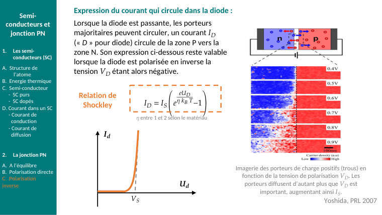
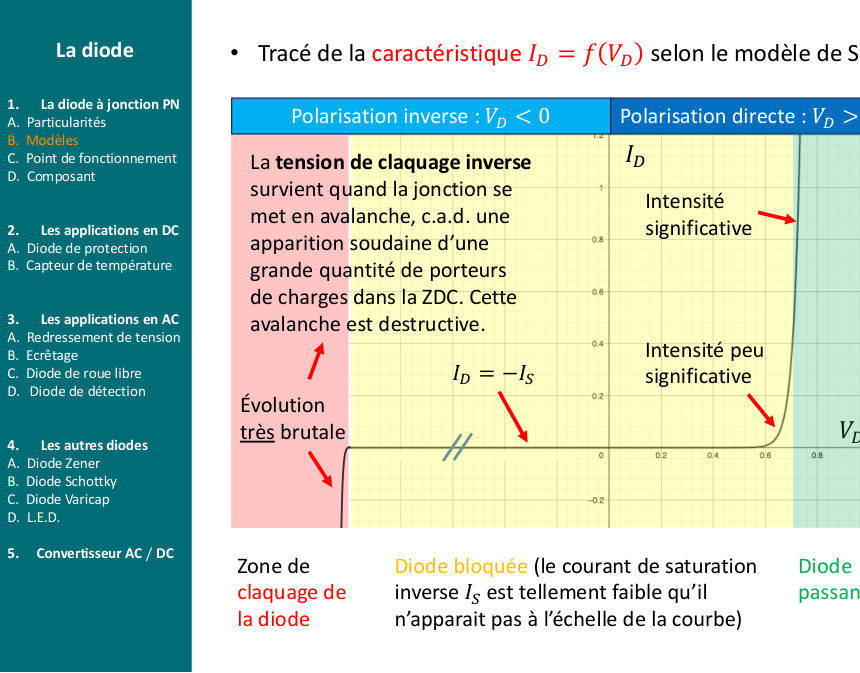
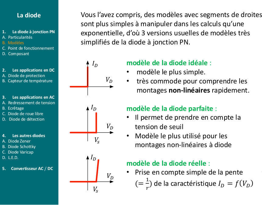
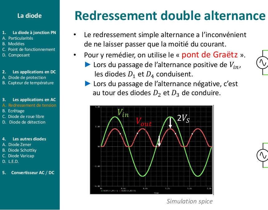
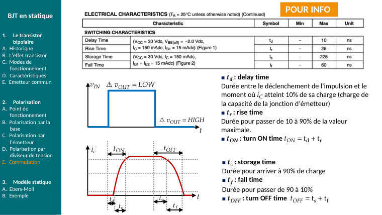
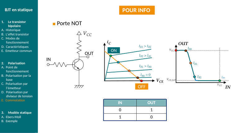
En électronique, 80 % de la réussite est dans les 30 premières secondes : reconnaître le type de problème et poser la bonne hypothèse.

Je vois dans l'énoncé…	… je fais
Un circuit à plusieurs sources, on demande un potentiel en un nœud	→Millman si toutes les branches arrivent au nœud, sinon méthode des nœuds. Superposition pour vérifier (\(V\to\) fil, \(I\to\) trou).
« Remplacer le circuit vu de \(A-B\) par… », « générateur équivalent », une charge variable \(R_{L}\)	→Thévenin : \(V_{\mathrm{Th}}\) = tension à vide (\(R_{L}\) enlevée), \(R_{\mathrm{Th}}\) = résistance vue de \(A-B\) sources neutralisées. Puis pont diviseur avec \(R_{L}\).
Un AOP avec une résistance qui relie la sortie à l'entrée −	→Contre-réaction ⟹ régime linéaire \(\Longrightarrow V_{+}=V_{-},\,\allowbreak i_{\pm }=0\). Loi des nœuds à l'entrée −. Vérifier ensuite \(\|V_{\mathrm{out}}\|\lt V_{\mathrm{sat}}\).
Un AOP sans contre-réaction (ou réaction sur +)	→Comparateur : \(V_{\mathrm{out}}=+V_{\mathrm{sat}}\) si \(V_{+}\gt V_{-}\), sinon \(-V_{\mathrm{sat}}\).
\(\rho ,\,\allowbreak \gamma ,\,\allowbreak \ell ,\,\allowbreak S\), « fil », « vitesse de dérive »	→\(R=\frac{\rho \ell }{S},\,\allowbreak i=\frac{u}{R},\,\allowbreak j=\frac{i}{S},\,\allowbreak E=\frac{u}{\ell },\,\allowbreak v=j\)/(ne) \(=\mu E\). Tout en SI \((m,\,\allowbreak m^{2},\,\allowbreak m^{-3})\).
\(N_{D},\,\allowbreak N_{A},\,\allowbreak n_{i}\), « dopé », « conductivité du silicium »	→Majoritaires ≈ dopage, minoritaires \(=n_{i}^{2}\)/dopage, \(\gamma =e(n\mu _{n}+p\mu _{p})\) (le terme minoritaire est négligeable). \(V_{0}=\left(\frac{kT}{e}\right)\cdot \ln \left(\frac{N_{A}N_{D}}{n_{i}^{2}}\right)\).
Une ou plusieurs diodes dans un circuit DC	→Hypothèse (bloquée ou passante) ⟹ calcul ⟹ vérification (bloquée : \(V_{D}\lt V_{S}\) ; passante : \(I_{D}\gt 0\)). Contradiction ⟹ changer d'hypothèse.
Une diode Zener, « régulateur », « \(R_{L,\,\mathrm{min}}\) », « \(V_{i,\,\mathrm{max}}\) »	→Loi des nœuds \(I_{R}=I_{Z}+I_{L}\) avec \(V_{\mathrm{out}}=V_{Z}\). Encadrer \(I_{Z}\) entre \(I_{Z,\,\mathrm{min}}\) et \(I_{Z,\,\mathrm{max}}\Longrightarrow\) bornes sur \(R_{L}\) ou \(V_{i}\).
Un signal sinusoïdal et des diodes (redresseur, écrêteur)	→Raisonner alternance par alternance : quelles diodes conduisent quand \(V_{\mathrm{in}}\gt 0\) ? quand \(V_{\mathrm{in}}\lt 0\) ? Tracer \(V_{\mathrm{out}}(t)\) avec la chute \(V_{S}\).
Un BJT et on demande « mode », « point de repos », « \(Q\) »	→Supposer actif : \(V_{\mathrm{BE}}=0{,}7\,\mathrm{V}\), maille de base \(\Longrightarrow I_{B},\,\allowbreak I_{C}=\beta I_{B}\), maille de collecteur \(\Longrightarrow V_{\mathrm{CE}}\). Vérifier \(V_{\mathrm{CE}}\gt 0{,}2\,\mathrm{V}\) (sinon saturé : \(I_{C}=I_{C,\,\mathrm{sat}}\)) et \(I_{B}\gt 0\) (sinon bloqué).
Un BJT polarisé par pont diviseur \(\frac{R_{1}}{R_{2}}+R_{E}\)	→Thévenin sur la base \((V_{\mathrm{Th}},\,\allowbreak R_{\mathrm{Th}})\), puis \(V_{E}=V_{\mathrm{Th}}-0{,}7,\,\allowbreak I_{E}=\frac{V_{E}}{R_{E}}\approx I_{C}\). Vérifier \(R_{\mathrm{Th}}\ll (\beta +1)R_{E}\).
« gain en tension », « impédance d'entrée », des condensateurs \(C_{1},\,\allowbreak C_{2},\,\allowbreak C_{3}\)	→Deux temps : DC (\(C\) ouverts) \(\Longrightarrow Q\Longrightarrow r_{E}=26\,\mathrm{mV}/I_{E}\). Puis AC (\(C\) = fils, sources DC = masse) \(\Longrightarrow A_{V}=\frac{-R_{C}}{r_{E}},\,\allowbreak Z_{\mathrm{in}},\,\allowbreak Z_{\mathrm{out}}\).
Un JFET avec \(R_{S}\) (autopolarisation)	→\(V_{\mathrm{GS}}=-R_{S}I_{D}\) injecté dans \(I_{D}=I_{\mathrm{DSS}}\left(1-\frac{V_{\mathrm{GS}}}{V_{\mathrm{GS},\,\mathrm{off}}}\right)^{2}\Longrightarrow\) équation \(\mathrm{d}u\,2^{\text{nd}}\) degré, garder la racine avec \(V_{\mathrm{GS},\,\mathrm{off}}\lt V_{\mathrm{GS}}\lt 0\).
Un MOSFET, on demande la région	→\(V_{\mathrm{GS}}\lt V_{T}\Longrightarrow\) bloqué. Sinon supposer saturé \(\left(I_{D}=\frac{1}{2}K_{n}\left(\frac{W}{L}\right)(V_{\mathrm{GS}}-V_{T})^{2}\right)\), calculer \(V_{\mathrm{DS}}\), vérifier \(V_{\mathrm{DS}}\ge V_{\mathrm{GS}}-V_{T}\). Sinon ohmique.
« Réaliser la fonction \(Y=\ldots\) en CMOS »	→PDN (nMOS) à partir de \(\bar{Y}\) sans complémenter les entrées : « + » = parallèle, « · » = série. PUN (pMOS) = structure duale (série ↔ parallèle) avec les mêmes entrées. Compter les transistors.
« délai », « chemin critique », \(R_{\square },\,\allowbreak C_{\square }\)	→\(R=R_{\square }\,\times\) nombre de carrés (coude \(=\frac{1}{2}\)), \(C_{\mathrm{OUT}}=\sum C_{\square }\cdot\)surface, \(\tau =\frac{(R_{N}+R_{P})C_{\mathrm{OUT}}}{2},\,\allowbreak n\) en série \(\Longrightarrow \left(\frac{n^{2}}{2}\right)\)RC. Le délai du circuit = le chemin le plus long.

◆ Les 5 réflexes avant de calculer

DC avant AC. Le point de repos d'abord (condensateurs ouverts), le petit signal ensuite (condensateurs = fils, sources DC = masse).
Hypothèse → calcul → vérification. Diode, transistor, AOP : on ne « devine » pas l'état, on le suppose puis on le contrôle. Une contradiction n'est pas une erreur, c'est une information.
Noter les valeurs par défaut : \(V_{S}=V_{\mathrm{BE}}=0{,}7\,\mathrm{V};\,\allowbreak V_{\mathrm{CE},\,\mathrm{sat}}\approx 0{,}2\,\mathrm{V};\,\allowbreak V_{T}=\frac{kT}{e}=26\,\mathrm{mV};\,\allowbreak \beta \approx 100-200\) sauf datasheet.
Ordres de grandeur : \(I_{B}\) en \(\mu A,\,\allowbreak I_{C}\) en \(mA,\,\allowbreak r_{E}\) en dizaines \(d'\Omega\), gains \(10-300,\,\allowbreak Z_{\mathrm{in}}\) en \(k\,\mathrm{\Omega }\) (BJT) ou \(M\,\mathrm{\Omega }\) (FET). Un résultat hors gamme ⟹ relire.
Unités SI : \(cm^{-3}\to m^{-3}\,(\times 10^{6}),\,\allowbreak \frac{cm^{2}}{V}\cdot s\to \frac{m^{2}}{V}\cdot s\,(\times 10^{-4}),\,\allowbreak mA\,\times \,k\,\mathrm{\Omega }=V\) (pratique), \(\mu A\,\times \,k\,\mathrm{\Omega }=mV\).

🔧 Les 14 déroulés

E1 Thévenin E2 AOP & dB E3 Fil & dérive E4 Dopage E5 Barrière \(V_{0}\)E6 Diode E7 Zener E8 BJT base E9 BJT pont E10 Gain AC E11 JFET E12 MOSFET E13 Porte CMOS E14 Délai

E1Ch. 0 · Thévenin

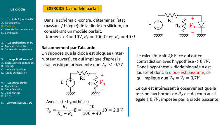
Pont diviseur chargé : \(V_{\mathrm{CC}}=12\,\mathrm{V},\,\allowbreak R_{1}=4\,\mathrm{k\Omega },\,\allowbreak R_{2}=8\,\mathrm{k\Omega }\), charge \(R_{L}=8\,\mathrm{k\Omega }\) aux bornes de \(R_{2}\)

Ce qu'on chercheLa tension \(V_{L}\) aux bornes de la charge. Piège : le diviseur de tension « nu » donne \(8\,\mathrm{V}\), mais la charge tire du courant et fait chuter la tension. Thévenin règle ça proprement.

Tension à vide (on enlève \(R_{L}\))
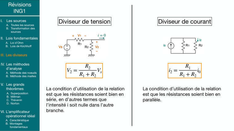
\(\displaystyle V_{\mathrm{Th}}=V_{\mathrm{CC}}\,\cdot \,\frac{R_{2}}{R_{1}+R_{2}}=12\,\cdot \,\frac{8}{12}=8\,\mathrm{V}\)
Résistance vue de \(A-B\), source neutralisée (\(V_{\mathrm{CC}}\to\) fil)
\(R_{1}\) et \(R_{2}\) se retrouvent en parallèle :
\(\displaystyle R_{\mathrm{Th}}=R_{1}//R_{2}=\frac{4\cdot 8}{4+8}=\frac{32}{12}\approx 2{,}67\,\mathrm{k\Omega }\)
Remettre la charge sur le générateur équivalent
\(\displaystyle V_{L}=V_{\mathrm{Th}}\,\cdot \,\frac{R_{L}}{R_{\mathrm{Th}}+R_{L}}=8\,\cdot \,\frac{8}{2{,}67+8}=8\,\cdot \,0{,}75=6\,\mathrm{V}\)
Contrôle sans Thévenin
\(R_{2}//R_{L}=4\,\mathrm{k\Omega }\), diviseur : \(12\,\cdot \,\frac{4}{4+4}=6\,\mathrm{V}\) ✓. Norton au passage : \(I_{N}=\frac{V_{\mathrm{Th}}}{R_{\mathrm{Th}}}=3\,\mathrm{mA}\).

Réponse\(V_{\mathrm{Th}}=8\,\mathrm{V},\,\allowbreak R_{\mathrm{Th}}=2{,}67\,\mathrm{k\Omega },\,\allowbreak V_{L}=6\,\mathrm{V}\) (et non \(8\,\mathrm{V}!\)).

Pourquoi ThéveninDès que la charge varie, on ne refait pas tout le circuit : on garde \((V_{\mathrm{Th}},\,\allowbreak R_{\mathrm{Th}})\) et on ne change que \(R_{L}\). Règle pratique : un pont diviseur se comporte en source de tension si \(R_{L}\gg R_{\mathrm{Th}}\) (ici \(8\,\mathrm{k}\) n'est pas \(\gg 2{,}67\,\mathrm{k}\), d'où la chute de 25 %).

E2Ch. 0 · AOP et décibels

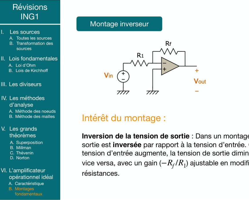
Non-inverseur \(R_{1}=1\,\mathrm{k\Omega },\,\allowbreak R_{f}=9\,\mathrm{k\Omega }\) ; puis inverseur \(R_{1}=2\,\mathrm{k\Omega },\,\allowbreak R_{f}=10\,\mathrm{k\Omega }\) ; alimentation \(\pm 15\,\mathrm{V}\)

Ce qu'on chercheLe gain de chaque montage, en linéaire et en dB, et la plage de \(V_{\mathrm{in}}\) pour laquelle l'AOP reste en régime linéaire.

Vérifier le régime
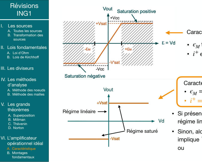
\(R_{f}\) relie la sortie à l'entrée − : contre-réaction négative ⟹ régime linéaire \(\Longrightarrow V_{+}=V_{-}\) et \(i_{\pm }=0\).
Non-inverseur : loi des nœuds à l'entrée −
\(V_{-}=V_{\mathrm{in}}\) est le point milieu du diviseur \(\frac{R_{1}}{R_{f}}\) alimenté par \(V_{\mathrm{out}}\) :
\(\displaystyle V_{\mathrm{in}}=V_{\mathrm{out}}\,\cdot \,\frac{R_{1}}{R_{1}+R_{f}}\Longrightarrow A=\frac{V_{\mathrm{out}}}{V_{\mathrm{in}}}=1+\frac{R_{f}}{R_{1}}=1+9=10\Longrightarrow 20\cdot \log (10)=20\,\mathrm{d}B\)
Inverseur : \(V_{-}=V_{+}=0\) (masse virtuelle)
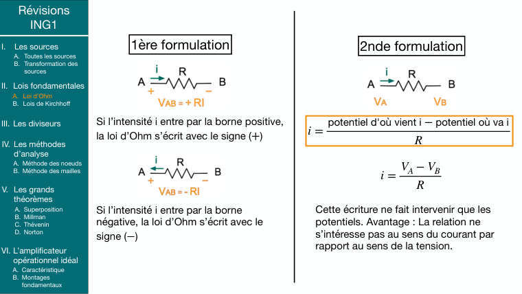
\(\displaystyle i=\frac{V_{\mathrm{in}}}{R_{1}}\text{ traverse }\,R_{f}\,(i_{-}=0)\colon V_{\mathrm{out}}=0-R_{f}\,\cdot \,i=-\left(\frac{R_{f}}{R_{1}}\right)\cdot V_{\mathrm{in}}=-5\cdot V_{\mathrm{in}}\) \(\displaystyle |A|=5\Longrightarrow 20\cdot \log (5)\approx 14\,\mathrm{d}B\,(\text{le signe }-\text{ est un déphasage de }\,180\text{°},\,\allowbreak \text{ pas un gain négatif en }\,\mathrm{d}B)\)
Plage linéaire
La sortie ne peut pas dépasser \(\pm V_{\mathrm{sat}}\approx \pm 15\,\mathrm{V}\) (souvent \(\pm 13-14\,\mathrm{V}\) en réel). Non-inverseur : \(|V_{\mathrm{in}}|\lt \frac{15}{10}=1{,}5\,\mathrm{V}\). Inverseur : \(|V_{\mathrm{in}}|\lt 3\,\mathrm{V}\). Au-delà, \(V_{\mathrm{out}}=\pm V_{\mathrm{sat}}\) (écrêtage).

Réponse\(A=+10\,(20\,\mathrm{d}B)\), linéaire pour \(|V_{\mathrm{in}}|\lt 1{,}5\,\mathrm{V};\,\allowbreak A=-5\,(14\,\mathrm{d}B)\), linéaire pour \(|V_{\mathrm{in}}|\lt 3\,\mathrm{V}\).

Table dB à connaître\(\times 1=0\,\mathrm{d}B,\,\allowbreak \times \sqrt{2}=3\,\mathrm{d}B,\,\allowbreak \times 2=6\,\mathrm{d}B,\,\allowbreak \times 10=20\,\mathrm{d}B,\,\allowbreak \times 100=40\,\mathrm{d}B\). Pour un gain en puissance c'est \(10\cdot \log\) (car \(P\,\propto \,V^{2}\)). Un gain \(0{,}5=-6\,\mathrm{d}B\) (atténuation).

E3Ch. 1 · Conduction

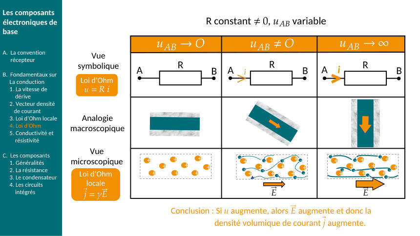
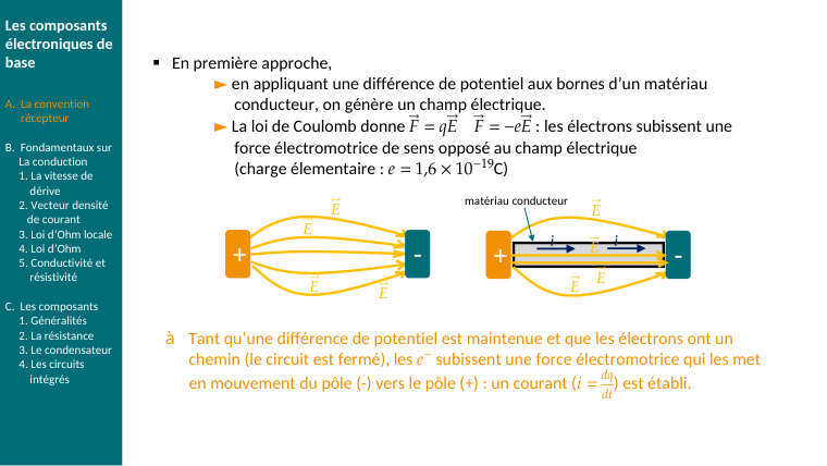
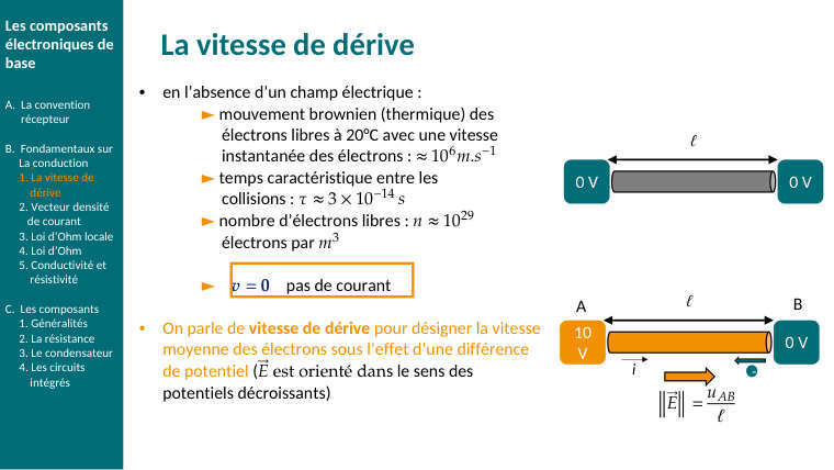
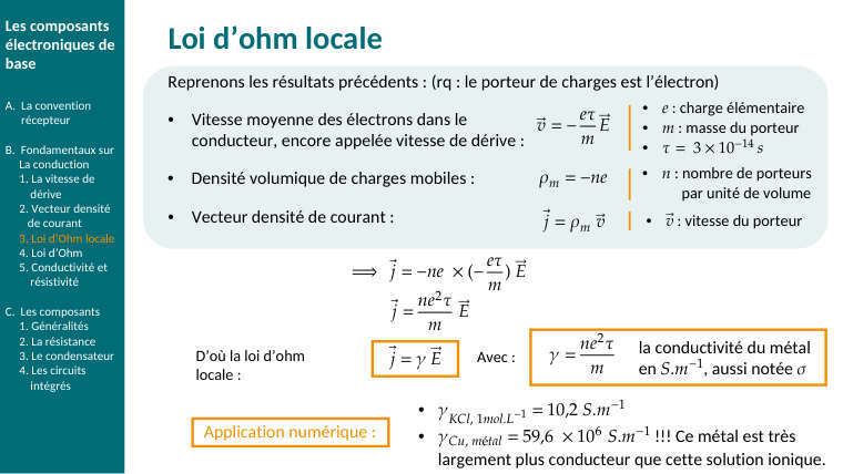
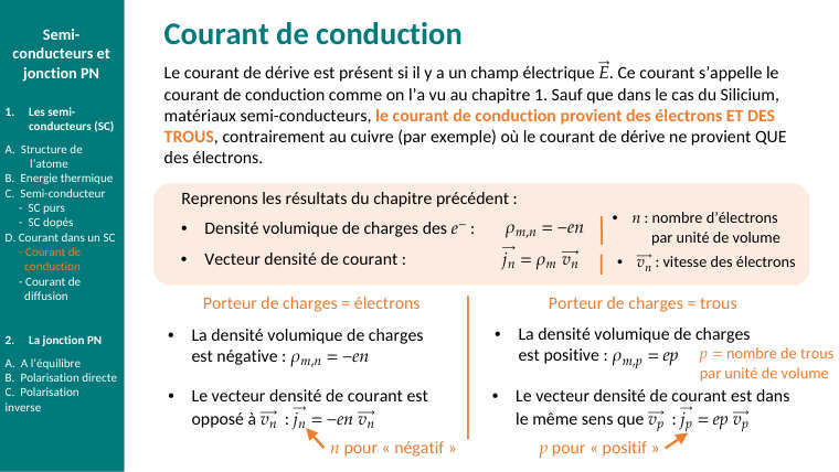
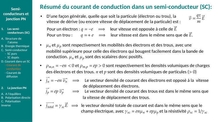
Fil de cuivre \(\ell =10\,\mathrm{m}\), diamètre \(1\,\mathrm{mm},\,\allowbreak \rho =1{,}7\cdot 10^{-8}\,\mathrm{\Omega }\cdot m\), parcouru par \(i=2\,\mathrm{A}\). Calculer \(R,\,\allowbreak u,\,\allowbreak j,\,\allowbreak E\) et la vitesse de dérive \((n=8{,}5\cdot 10^{28}\,\mathrm{m}^{-3})\).

Ce qu'on chercheUne chaîne de formules, chacune à une ligne. Le seul danger : les unités (mm \(\to m\), section \(=\pi r^{2}\) avec le rayon).

Section et résistance
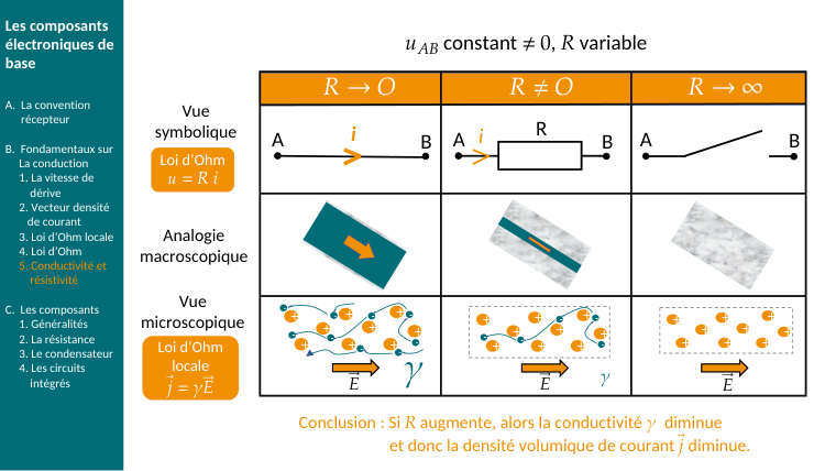
\(\displaystyle S=\pi \,r^{2}=\pi \,(0{,}5\cdot 10^{-3})^{2}=7{,}85\cdot 10^{-7}\,\mathrm{m}^{2}\) \(\displaystyle R=\rho \,\ell \,/\,S=1{,}7\cdot 10^{-8}\,\cdot \,10\,/\,7{,}85\cdot 10^{-7}\approx 0{,}22\,\mathrm{\Omega }\)
Tension, champ, densité de courant
\(\displaystyle u=R\,i=0{,}22\,\cdot \,2\approx 0{,}43\,\mathrm{V}\,E=\frac{u}{\ell }=0{,}043\,\mathrm{V}/\,\mathrm{m}\) \(\displaystyle j=\frac{i}{S}=2\,/\,7{,}85\cdot 10^{-7}\approx 2{,}5\cdot 10^{6}\,\mathrm{A}/\,\mathrm{m}^{2}\,\left(\text{vérif }\colon j=\gamma E=\left(\frac{1}{\rho }\right)\cdot E=5{,}9\cdot 10^{7}\,\cdot \,0{,}043\approx 2{,}5\cdot 10^{6}\text{ ✓}\right)\)
Vitesse de dérive
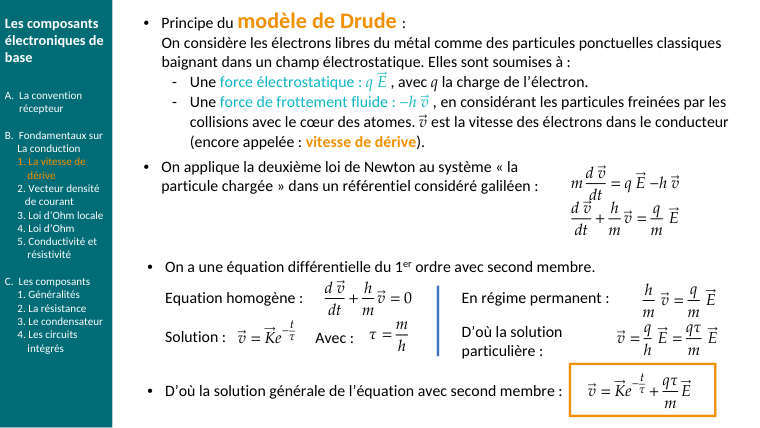
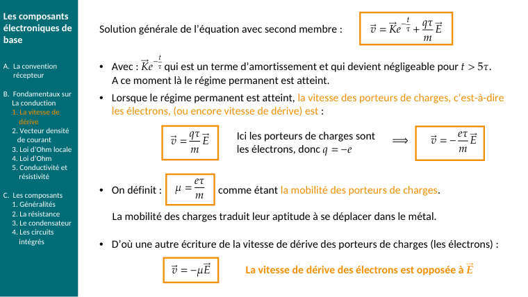
\(\displaystyle j=n\,e\,v\Longrightarrow v=\frac{j}{(n\,e)}=2{,}5\cdot 10^{6}\,/\,(8{,}5\cdot 10^{28}\,\cdot \,1{,}6\cdot 10^{-19})=2{,}5\cdot 10^{6}\,/\,1{,}36\cdot 10^{10}\approx 1{,}9\cdot 10^{-4}\,\mathrm{m}/\,\mathrm{s}\approx 0{,}2\,\mathrm{mm}/\,\mathrm{s}\)
Mobilité (bonus)
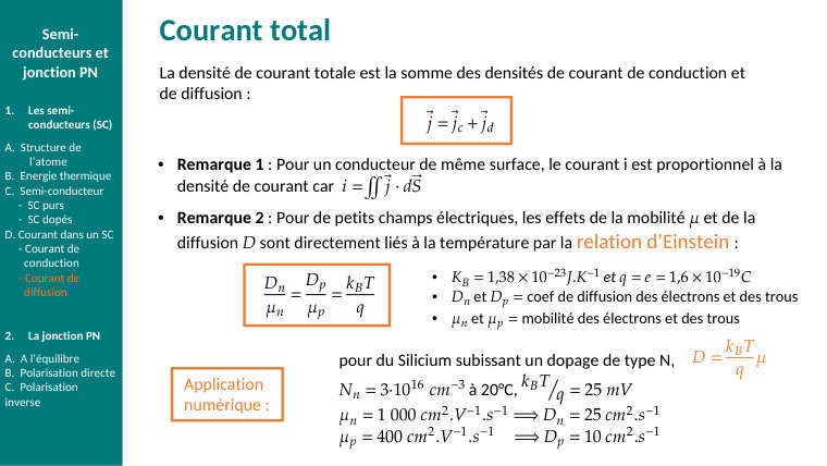
\(v=\mu E\Longrightarrow \mu =\frac{v}{E}=1{,}9\cdot \frac{10^{-4}}{0{,}043}\approx 4{,}3\cdot 10^{-3}\,\mathrm{m}^{2}/V\cdot s\). Ordre de grandeur correct pour le cuivre.

Réponse\(R\approx 0{,}22\,\mathrm{\Omega };\,\allowbreak u\approx 0{,}43\,\mathrm{V};\,\allowbreak j\approx 2{,}5\cdot 10^{6}\,\mathrm{A}/\,\mathrm{m}^{2};\,\allowbreak v\approx 0{,}2\,\mathrm{mm}/\,\mathrm{s}\).

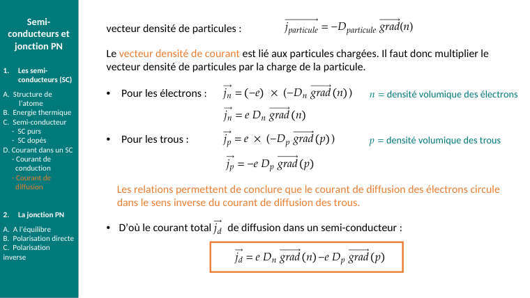
L'ordre de grandeur à retenirLa vitesse de dérive des électrons est de l'ordre du \(\frac{mm}{s}\) alors que le signal se propage quasi à la vitesse de la lumière : ce qui se propage, c'est le champ \(E\), pas les électrons.

E4Ch. 2 · Dopage

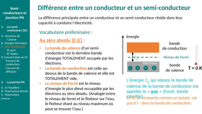
Silicium dopé au phosphore \(N_{D}=10^{16}\,\mathrm{cm}^{-3}\) à \(300\,\mathrm{K}\,(n_{i}=1{,}5\cdot 10^{10}\,\mathrm{cm}^{-3},\,\allowbreak \mu _{n}=1350,\,\allowbreak \mu _{p}=480\,\mathrm{cm}^{2}/V\cdot s)\)

Ce qu'on chercheLe type, les densités \(n\) et \(p\), la conductivité et la résistivité. Puis comparer au silicium intrinsèque.

Identifier
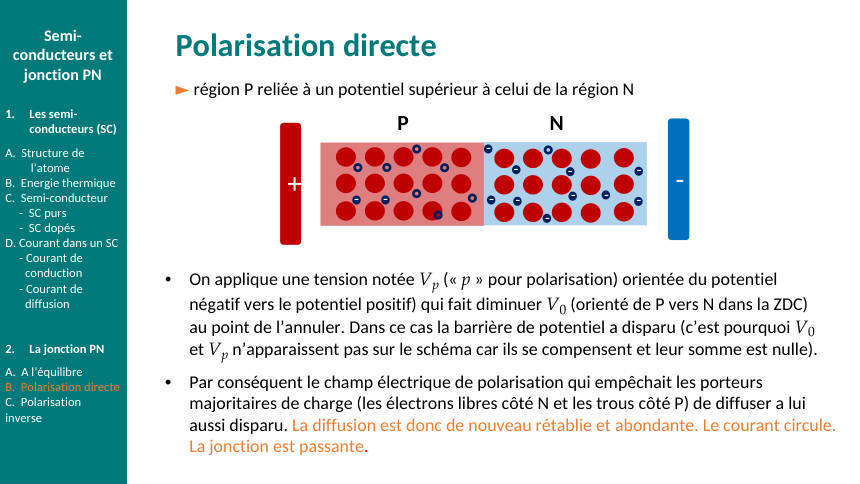
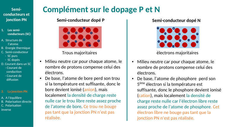
Phosphore : groupe \(V,\,\allowbreak 5\) électrons de valence ⟹ donneur ⟹ type \(\mathbf{N}\), électrons majoritaires.
Densités \((N_{D}\gg n_{i})\)
\(\displaystyle n\approx N_{D}=10^{16}\,\mathrm{cm}^{-3}\) \(\displaystyle p=\frac{n_{i}^{2}}{N_{D}}=(1{,}5\cdot 10^{10})^{2}\,/\,10^{16}=2{,}25\cdot 10^{20}\,/\,10^{16}=2{,}25\cdot 10^{4}\,\mathrm{cm}^{-3}\)
Rapport \(\frac{n}{p}\approx 4\cdot 10^{11}\) : les trous sont totalement négligeables.
Conductivité (en unités cm : \(e\) en \(C,\,\allowbreak n\) en \(cm^{-3},\,\allowbreak \mu\) en \(\frac{cm^{2}}{V}\cdot s\Longrightarrow \gamma\) en \(\frac{S}{cm}\))
\(\displaystyle \gamma =e\,(n\,\mu _{n}+p\,\mu _{p})\approx 1{,}6\cdot 10^{-19}\,\cdot \,10^{16}\,\cdot \,1350\approx 2{,}2\,\mathrm{S}/cm\Longrightarrow \rho =\frac{1}{\gamma }\approx 0{,}46\,\mathrm{\Omega }\cdot \text{cm}\)
Comparaison avec l'intrinsèque
\(\displaystyle \gamma _{i}=e\,n_{i}\,(\mu _{n}+\mu _{p})=1{,}6\cdot 10^{-19}\,\cdot \,1{,}5\cdot 10^{10}\,\cdot \,1830\approx 4{,}4\cdot 10^{-6}\,\mathrm{S}/cm\)
Le dopage à 1 atome pour ~5 millions (\(10^{16}\,/\,5\cdot 10^{22}\) atomes de Si) multiplie la conductivité par ~500 000. C'est tout le principe du semi-conducteur.

RéponseType \(N;\,\allowbreak n=10^{16}\,\mathrm{cm}^{-3},\,\allowbreak p=2{,}25\cdot 10^{4}\,\mathrm{cm}^{-3};\,\allowbreak \gamma \approx 2{,}2\,\mathrm{S}/cm,\,\allowbreak \rho \approx 0{,}46\,\mathrm{\Omega }\cdot\)cm.

Piège d'unitésSi l'énoncé mélange \(cm^{-3}\) et \(\frac{m^{2}}{V}\cdot s\), tout convertir : \(10^{16}\,\mathrm{cm}^{-3}=10^{22}\,\mathrm{m}^{-3};\,\allowbreak 1350\,\mathrm{cm}^{2}/V\cdot s=0{,}135\,\mathrm{m}^{2}/V\cdot s\). Alors \(\gamma =1{,}6\cdot 10^{-19}\,\cdot \,10^{22}\,\cdot \,0{,}135=216\,\mathrm{S}/\,\mathrm{m}=2{,}16\,\mathrm{S}/cm\) ✓ \((1\,\mathrm{S}/cm=100\,\mathrm{S}/\,\mathrm{m})\).

E5Ch. 2 · Jonction PN

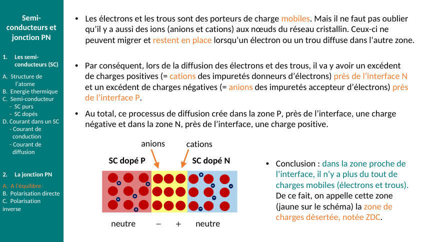
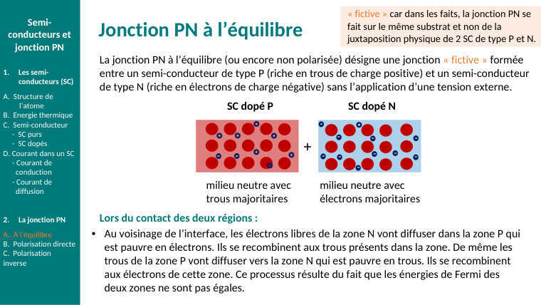
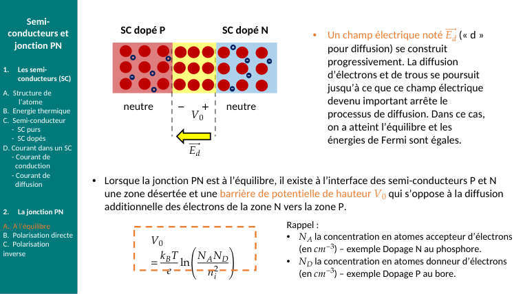
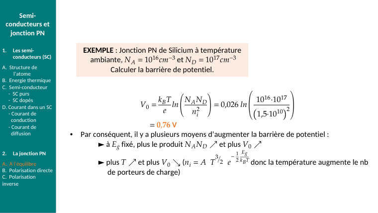
Barrière de potentiel d'une jonction Si avec \(N_{A}=10^{17}\,\mathrm{cm}^{-3},\,\allowbreak N_{D}=10^{16}\,\mathrm{cm}^{-3}\) à \(300\,\mathrm{K}\)

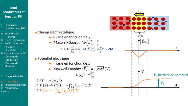
Ce qu'on cherche\(V_{0}\), puis l'effet d'une hausse de température et d'un dopage plus fort. Formule : \(V_{0}=\left(\frac{k_{B}T}{e}\right)\cdot \ln \left(\frac{N_{A}N_{D}}{n_{i}^{2}}\right)\).

Tension thermique
\(\displaystyle k_{B}\,T\,/\,e=1{,}38\cdot 10^{-23}\,\cdot \,300\,/\,1{,}6\cdot 10^{-19}\approx 0{,}026\,\mathrm{V}=26\,\mathrm{mV}\)
À retenir par cœur, c'est aussi le \(V_{T}\) de \(r_{E}=26\,\mathrm{mV}/I_{E}\).
Argument du logarithme
\(\displaystyle N_{A}\,N_{D}\,/\,n_{i}^{2}=10^{17}\,\cdot \,10^{16}\,/\,(1{,}5\cdot 10^{10})^{2}=10^{33}\,/\,2{,}25\cdot 10^{20}\approx 4{,}4\cdot 10^{12}\) \(\displaystyle \ln (4{,}4\cdot 10^{12})=\ln \,4{,}4+12\cdot \ln \,10\approx 1{,}48+27{,}6\approx 29{,}1\)
Barrière
\(\displaystyle V_{0}=0{,}026\,\cdot \,29{,}1\approx 0{,}76\,\mathrm{V}\)
Cohérent avec la valeur « typique » du cours et proche du seuil \(0{,}7\,\mathrm{V}\) de la diode.
Variations
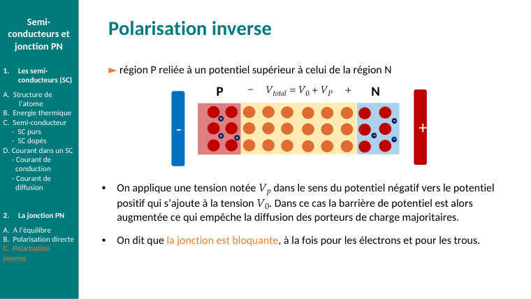
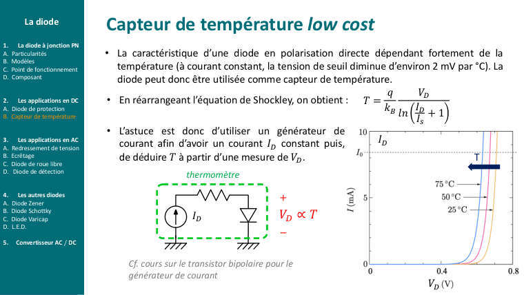
Dopage \(\times 10\) sur \(N_{D}\Longrightarrow \ln\) augmente de \(\ln \,10=2{,}3\Longrightarrow V_{0}+60\,\mathrm{mV}\). \(T\) qui monte \(\Longrightarrow n_{i}\) explose \(\left(e^{\frac{-E_{g}}{2}\,\mathrm{kT}}\right)\Longrightarrow\) l'argument \(\mathrm{d}u\,\ln\) chute plus vite que \(\frac{kT}{e}\) ne monte ⟹ \(V_{0}\) diminue (\(\approx -2\,\mathrm{mV}/^{\circ}\mathrm{C}\), c'est le capteur de température à diode).

Réponse\(V_{0}\approx 0{,}76\,\mathrm{V}\).

Calculer un \(\ln\) sans calculatrice\(\ln (a\cdot 10^{k})=\ln \,a+2{,}3\cdot k\). Avec \(\ln \,2\approx 0{,}69,\,\allowbreak \ln \,3\approx 1{,}1,\,\allowbreak \ln \,5\approx 1{,}6\), on encadre n'importe quel logarithme à 5 % près.

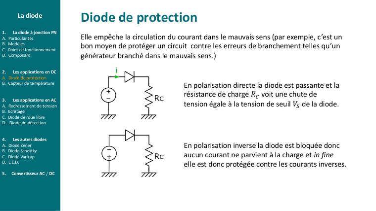
E6Ch. 3 · État d'une diode

Source \(E\) en série avec \(R=1\,\mathrm{k\Omega }\) et une diode Si. Cas \((a)\,E=5\,\mathrm{V}\) dans le sens passant ; \((b)\,E=0{,}5\,\mathrm{V};\,\allowbreak (c)\,E=5\,\mathrm{V}\), diode retournée. Modèle parfait, puis réel avec \(r=10\,\mathrm{\Omega }\).

Ce qu'on chercheL'état de la diode et le point de fonctionnement \((V_{D},\,\allowbreak I_{D})\) dans chaque cas, par la méthode de l'hypothèse.

(a) Hypothèse « bloquée »
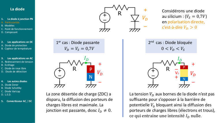
\(I_{D}=0\Longrightarrow\) pas de chute dans \(R\Longrightarrow V_{D}=E=5\,\mathrm{V}\). Or une diode bloquée doit avoir \(V_{D}\lt 0{,}7\,\mathrm{V}\) : contradiction ⟹ elle est passante.
(a) Hypothèse « passante », modèle parfait \(V_{D}=0{,}7\,\mathrm{V}\)
\(\displaystyle \text{Maille }\colon E-R\,I_{D}-V_{S}=0\Longrightarrow I_{D}=\frac{E-V_{S}}{R}=\frac{5-0{,}7}{1000}=4{,}3\,\mathrm{mA}\gt 0\text{ ✓ cohérent}\)
(a) Modèle réel
\(\displaystyle I_{D}=\frac{E-V_{S}}{R+r}=\frac{4{,}3}{1010}\approx 4{,}26\,\mathrm{mA};\,\allowbreak V_{D}=V_{S}+r\,I_{D}=0{,}7+0{,}043\approx 0{,}74\,\mathrm{V}\)
Différence de 1 % : le modèle parfait suffit dès que \(R\gg r\).
\((b)\,E=0{,}5\,\mathrm{V}\)
Hypothèse bloquée : \(V_{D}=0{,}5\,\mathrm{V}\lt 0{,}7\,\mathrm{V}\) ✓ cohérent ⟹ bloquée, \(I_{D}=0,\,\allowbreak V_{R}=0\). (Hypothèse passante donnerait \(I_{D}=\frac{0{,}5-0{,}7}{R}\lt 0\) : absurde.)
\((c)\) Diode en inverse
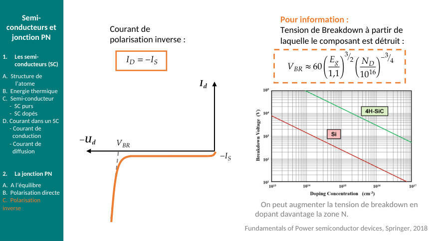
Hypothèse bloquée : \(V_{D}=-5\,\mathrm{V}\lt 0{,}7\) ✓ ⟹ bloquée. Vérifier que \(|-5\,\mathrm{V}|\lt V_{\mathrm{BR}}\) (ex. \(100\,\mathrm{V}\) pour une 1N4148) : pas de claquage. Toute la tension \(E\) est aux bornes de la diode.

Réponse(a) passante, \(I_{D}=4{,}3\,\mathrm{mA},\,\allowbreak V_{D}=0{,}7\,\mathrm{V}\) (\(0{,}74\,\mathrm{V}\) en réel) ; \((b)\) bloquée ; \((c)\) bloquée, \(V_{D}=-5\,\mathrm{V}\).

Avec plusieurs diodesMême méthode : on suppose un état pour chaque diode (2 diodes = 4 combinaisons), on calcule, on vérifie toutes les conditions. Commencer par l'hypothèse la plus plausible (celle où la source « pousse » dans le sens passant).

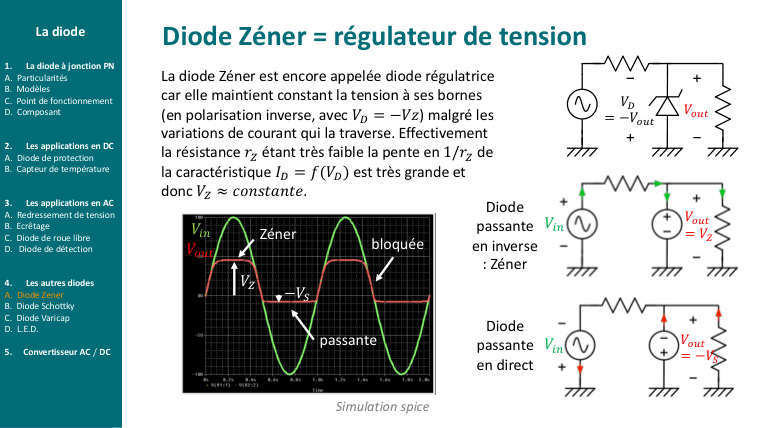
E7Ch. 3 · Régulateur Zener

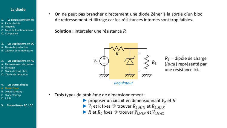
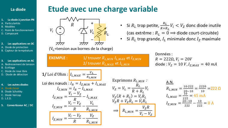
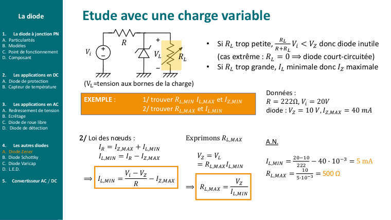
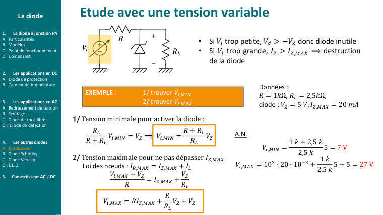
\(V_{i}=12\,\mathrm{V},\,\allowbreak R=220\,\mathrm{\Omega },\,\allowbreak V_{Z}=5{,}1\,\mathrm{V},\,\allowbreak I_{Z,\,\mathrm{max}}=50\,\mathrm{mA},\,\allowbreak I_{Z,\,\mathrm{min}}=1\,\mathrm{mA}\). Charge \(R_{L}\) variable.

Ce qu'on cherche(1) Vérifier que la Zener survit sans charge. \((2)\,R_{L,\,\mathrm{min}}\) pour rester régulé. (3) Puissance dans \(R\) et dans la Zener.

Courant dans \(R\) (constant tant que la régulation tient)
\(\displaystyle I_{R}=\frac{V_{i}-V_{Z}}{R}=\frac{12-5{,}1}{220}=\frac{6{,}9}{220}\approx 31{,}4\,\mathrm{mA}\)
Sans charge : tout passe dans la Zener
\(I_{Z}=I_{R}=31{,}4\,\mathrm{mA}\lt I_{Z,\,\mathrm{max}}=50\,\mathrm{mA}\) ✓. Puissance dissipée : \(P_{Z}=5{,}1\,\cdot \,0{,}0314\approx 0{,}16\,\mathrm{W}\) (choisir une Zener \(0{,}5\,\mathrm{W}\)).
Avec charge : loi des nœuds
\(\displaystyle I_{R}=I_{Z}+I_{L}\Longrightarrow I_{L}=I_{R}-I_{Z}\) \(\displaystyle \text{Régulation maintenue tant que }\,I_{Z}\ge I_{Z,\,\mathrm{min}}\Longrightarrow I_{L}\le I_{R}-I_{Z,\,\mathrm{min}}=31{,}4-1=30{,}4\,\mathrm{mA}\) \(\displaystyle R_{L,\,\mathrm{min}}=V_{Z}\,/\,I_{L,\,\mathrm{max}}=5{,}1\,/\,0{,}0304\approx 168\,\mathrm{\Omega }\)
Formule du cours \((I_{Z,\,\mathrm{min}}=0)\)
\(\displaystyle R_{L,\,\mathrm{min}}=V_{Z}\,\cdot \,R\,/\,(V_{i}-V_{Z})=5{,}1\,\cdot \,220\,/\,6{,}9\approx 163\,\mathrm{\Omega }\)
Même résultat à 3 % près ; la version avec \(I_{Z,\,\mathrm{min}}\) est plus sûre.
Si \(R_{L}\lt R_{L,\,\mathrm{min}}\) ?
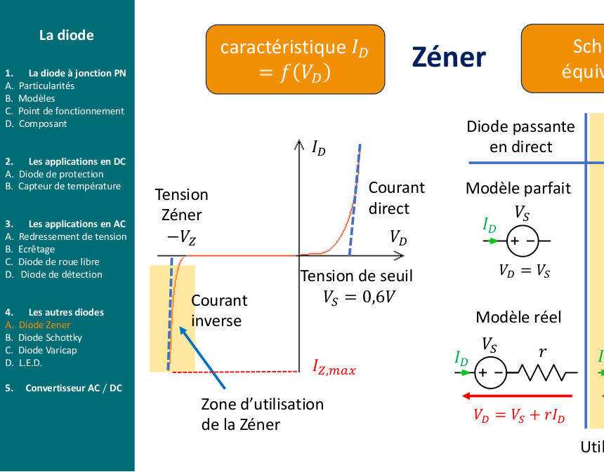
La Zener se bloque \((I_{Z}=0)\), le circuit redevient un simple diviseur \(\frac{R}{R_{L}}\colon V_{\mathrm{out}}=12\cdot \frac{R_{L}}{220+R_{L}}\lt 5{,}1\,\mathrm{V}\). Plus de régulation.

Réponse\(I_{R}\approx 31\,\mathrm{mA}\) ; sans charge OK \((P_{Z}\approx 0{,}16\,\mathrm{W});\,\allowbreak R_{L,\,\mathrm{min}}\approx 165-170\,\mathrm{\Omega }\).

Le raisonnement en « budget de courant »\(R\) fournit un courant fixe \(I_{R}\). La charge en prend ce qu'elle veut, la Zener absorbe le reste. Quand le reste devient nul, la régulation lâche. Le problème inverse (\(V_{i}\) variable, \(R_{L}\) fixe) se traite pareil : \(V_{i,\,\mathrm{min}}\) tel que \(I_{R}\ge I_{L}+I_{Z,\,\mathrm{min}},\,\allowbreak V_{i,\,\mathrm{max}}\) tel que \(I_{R}\le I_{L}+I_{Z,\,\mathrm{max}}\).

E8Ch. 4 · Polarisation par la base

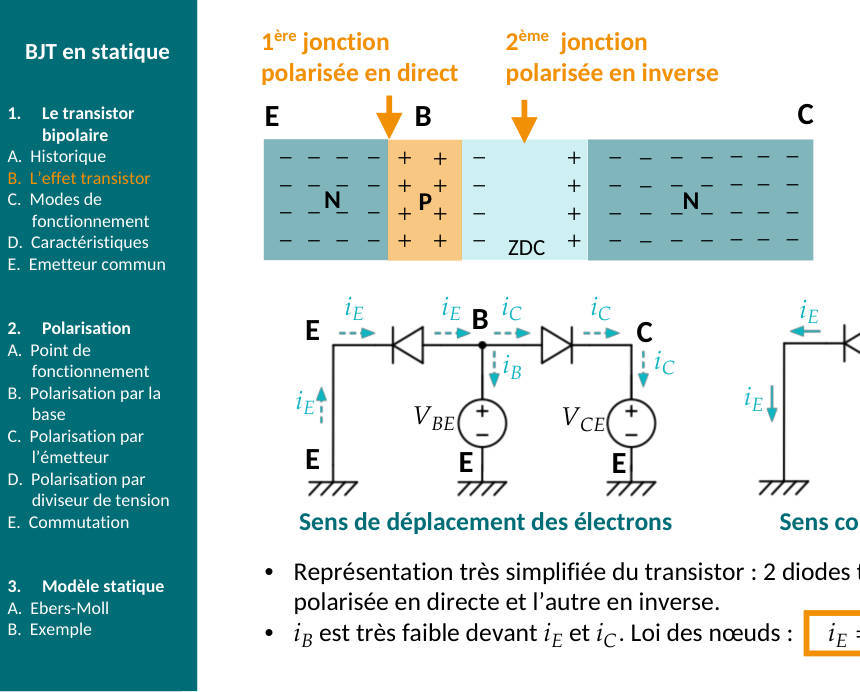
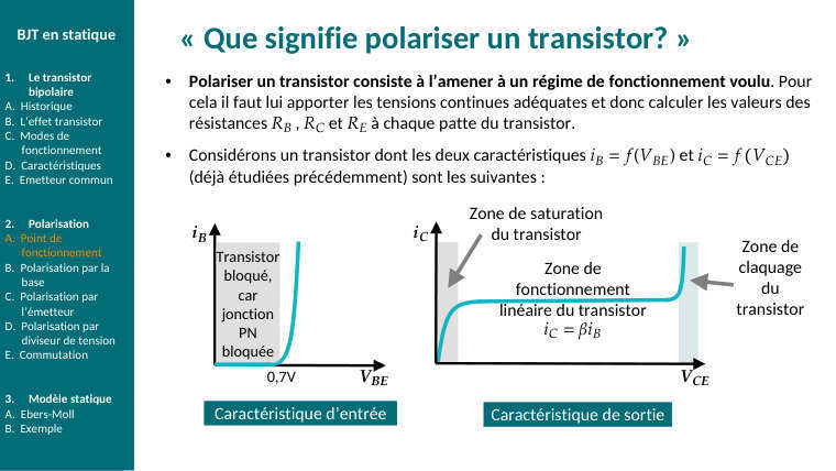
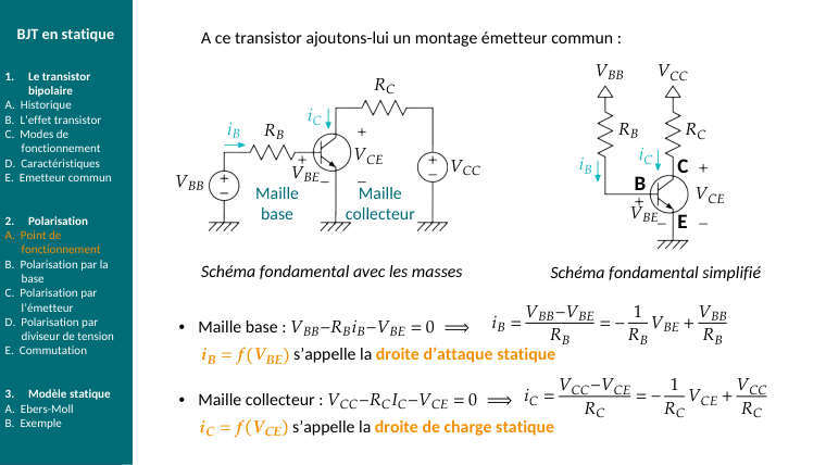
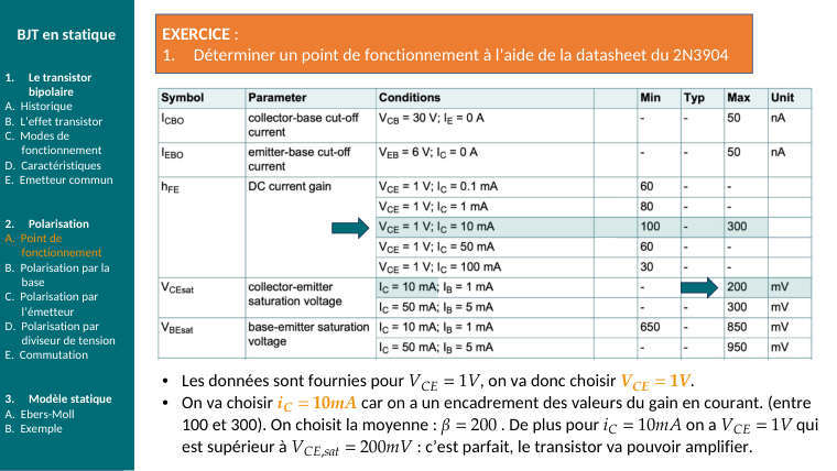
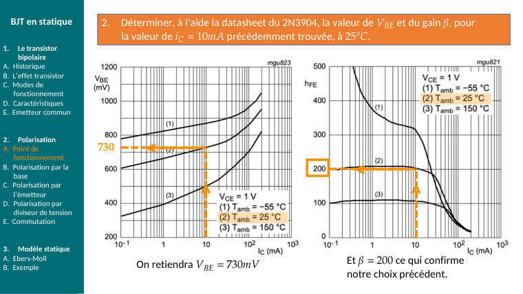
\(V_{\mathrm{CC}}=12\,\mathrm{V},\,\allowbreak V_{\mathrm{BB}}=5\,\mathrm{V},\,\allowbreak R_{B}=100\,\mathrm{k\Omega },\,\allowbreak R_{C}=1\,\mathrm{k\Omega }\). Point \(Q\) pour \(\beta =100\), puis \(\beta =300\).

Ce qu'on cherche\((I_{B},\,\allowbreak I_{C},\,\allowbreak V_{\mathrm{CE}})\) et le mode. Puis montrer pourquoi cette polarisation est « \(\beta\)-dépendante ».

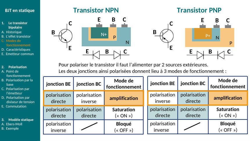
Hypothèse : mode actif, \(V_{\mathrm{BE}}=0{,}7\,\mathrm{V}\). Maille de base
\(\displaystyle I_{B}=\frac{V_{\mathrm{BB}}-V_{\mathrm{BE}}}{R_{B}}=\frac{5-0{,}7}{100}\,\mathrm{k}=43\,\mu A\)
Courant de collecteur et maille de collecteur \((\beta =100)\)
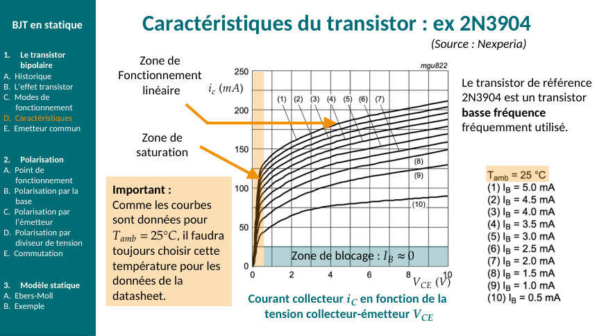
\(\displaystyle I_{C}=\beta \,I_{B}=4{,}3\,\mathrm{mA}\) \(\displaystyle V_{\mathrm{CE}}=V_{\mathrm{CC}}-R_{C}\,I_{C}=12-1\,\mathrm{k}\,\cdot \,4{,}3\,\mathrm{m}=7{,}7\,\mathrm{V}\gt 0{,}2\,\mathrm{V}\text{ ✓ mode actif confirmé}\)
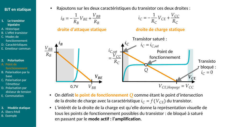
Droite de charge et saturation
\(\displaystyle I_{C,\,\mathrm{sat}}=V_{\mathrm{CC}}\,/\,R_{C}=12\,\mathrm{mA}\,(\text{à }\,V_{\mathrm{CE}}\approx 0)\)
\(Q=(7{,}7\,\mathrm{V};\,\allowbreak 4{,}3\,\mathrm{mA})\) est à peu près au milieu de la droite de charge : bon pour amplifier.
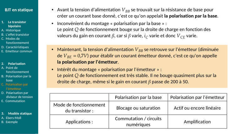
Même circuit, \(\beta =300\) (autre exemplaire, ou \(T\) plus élevée)
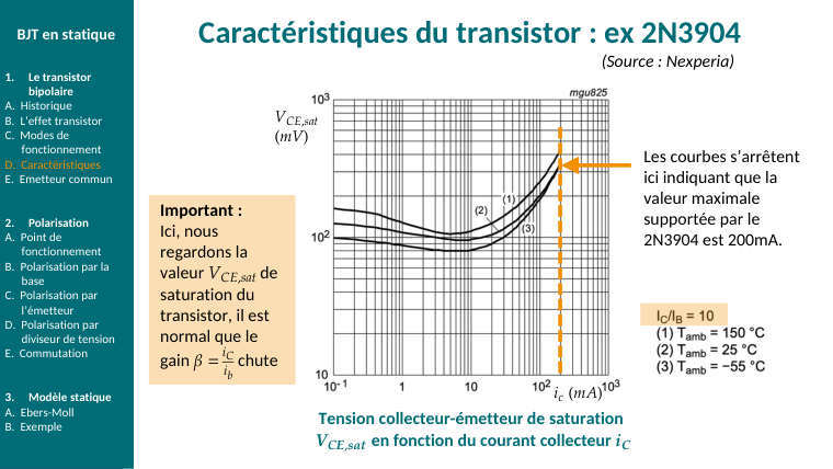
\(\displaystyle I_{C}=300\,\cdot \,43\,\mu =12{,}9\,\mathrm{mA}\gt I_{C,\,\mathrm{sat}}=12\,\mathrm{mA}\Longrightarrow \text{ IMPOSSIBLE }\Longrightarrow \text{ transistor SATURÉ}\) \(\displaystyle \text{On plafonne }\colon I_{C}=I_{C,\,\mathrm{sat}}\approx 12\,\mathrm{mA},\,\allowbreak V_{\mathrm{CE}}=V_{\mathrm{CE},\,\mathrm{sat}}\approx 0{,}1-0{,}2\,\mathrm{V}\)

Réponse\(\beta =100\) : actif, \(Q=(7{,}7\,\mathrm{V};\,\allowbreak 4{,}3\,\mathrm{mA})\). \(\beta =300\) : saturé, \(V_{\mathrm{CE}}\approx 0{,}2\,\mathrm{V}\). Le point \(Q\) dépend de \(\beta \Longrightarrow\) mauvaise polarisation pour un ampli, très bien pour un interrupteur.

Le test de saturation, toujoursAprès \(I_{C}=\beta I_{B}\), comparer à \(I_{C,\,\mathrm{sat}}\). Un \(V_{\mathrm{CE}}\) négatif dans la maille de collecteur est le signal d'alarme : ça veut dire « saturé ». En commutation on veut \(\beta \cdot I_{B}\gg I_{C,\,\mathrm{sat}}\) (facteur 2 à 10 de sécurité).

E9Ch. 4 · Polarisation par pont diviseur

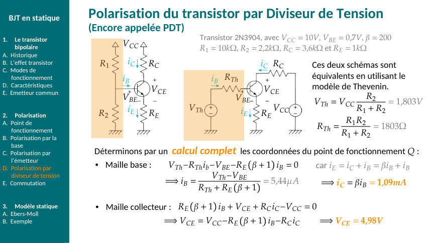
\(V_{\mathrm{CC}}=12\,\mathrm{V},\,\allowbreak R_{1}=10\,\mathrm{k\Omega },\,\allowbreak R_{2}=2{,}2\,\mathrm{k\Omega },\,\allowbreak R_{E}=2{,}2\,\mathrm{k\Omega },\,\allowbreak R_{C}=3{,}3\,\mathrm{k\Omega },\,\allowbreak \beta =150\)

Ce qu'on chercheLe point \(Q\) par la méthode Thévenin-sur-la-base, la vérification de la condition de « vraie source », et pourquoi \(Q\) ne dépend presque plus de \(\beta\).

Thévenin vu de la base
\(\displaystyle V_{\mathrm{Th}}=V_{\mathrm{CC}}\,\cdot \,\frac{R_{2}}{R_{1}+R_{2}}=12\,\cdot \,\frac{2{,}2}{12{,}2}\approx 2{,}16\,\mathrm{V}\) \(\displaystyle R_{\mathrm{Th}}=R_{1}//R_{2}=10\cdot \frac{2{,}2}{12{,}2}\approx 1{,}80\,\mathrm{k\Omega }\)
Condition de stabilité
\(\displaystyle R_{\mathrm{Th}}\lt 0{,}01\cdot (\beta +1)\cdot R_{E}=0{,}01\,\cdot \,151\,\cdot \,2{,}2\,\mathrm{k}=3{,}32\,\mathrm{k\Omega }\Longrightarrow 1{,}80\,\mathrm{k}\lt 3{,}32\,\mathrm{k}\text{ ✓}\)
Le pont se comporte comme une vraie source de tension : le courant de base ne le « charge » pas.
Méthode rapide (\(\beta\)-indépendante)
\(\displaystyle V_{E}=V_{\mathrm{Th}}-V_{\mathrm{BE}}=2{,}16-0{,}7=1{,}46\,\mathrm{V}\) \(\displaystyle I_{E}=V_{E}\,/\,R_{E}=1{,}46\,/\,2{,}2\,\mathrm{k}\approx 0{,}66\,\mathrm{mA}\approx I_{C}\) \(\displaystyle V_{C}=V_{\mathrm{CC}}-R_{C}\,I_{C}=12-3{,}3\,\mathrm{k}\,\cdot \,0{,}66\,\mathrm{m}\approx 9{,}8\,\mathrm{V}\) \(\displaystyle V_{\mathrm{CE}}=V_{C}-V_{E}\approx 9{,}8-1{,}46\approx 8{,}4\,\mathrm{V}\gt 0{,}2\text{ ✓ actif}\)
Méthode exacte (pour voir l'écart)
\(\displaystyle \text{Maille base }\colon V_{\mathrm{Th}}-R_{\mathrm{Th}}\,I_{B}-V_{\mathrm{BE}}-R_{E}\,(\beta +1)\,I_{B}=0\) \(\displaystyle I_{B}=1{,}46\,/\,(1{,}8\,\mathrm{k}+151\,\cdot \,2{,}2\,\mathrm{k})=1{,}46\,/\,334\,\mathrm{k}\approx 4{,}4\,\mu A\Longrightarrow I_{C}=150\,\cdot \,4{,}4\,\mu \approx 0{,}66\,\mathrm{mA}\)
Identique à 1 % près. Avec \(\beta =300\colon I_{B}=\frac{1{,}46}{(1{,}8\,\mathrm{k}+662\,\mathrm{k})}=2{,}2\,\mu A,\,\allowbreak I_{C}=0{,}66\,\mathrm{mA}\) — inchangé. C'est tout l'intérêt de \(R_{E}\).

Réponse\(Q\approx (V_{\mathrm{CE}}=8{,}4\,\mathrm{V};\,\allowbreak I_{C}=0{,}66\,\mathrm{mA})\), stable en \(\beta\).

Pourquoi \(R_{E}\) stabiliseSi \(\beta\) augmente, \(I_{C}\) veut augmenter \(\Longrightarrow V_{E}=R_{E}I_{E}\) augmente \(\Longrightarrow V_{\mathrm{BE}}=V_{B}-V_{E}\) diminue \(\Longrightarrow I_{B}\) diminue \(\Longrightarrow I_{C}\) revient. C'est une contre-réaction, comme dans l'AOP.

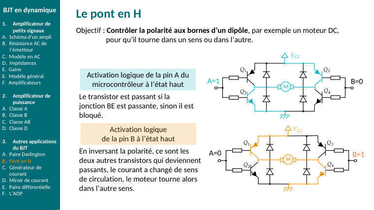
E10Ch. 5 · Émetteur commun en AC

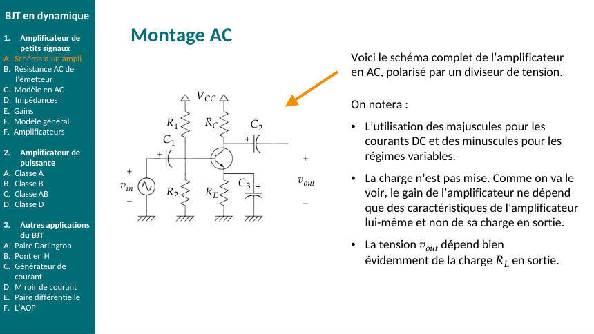
Même montage que E9 \((I_{E}=0{,}66\,\mathrm{mA})\), avec \(C_{1},\,\allowbreak C_{2}\) de liaison et \(C_{3}\) de découplage sur \(R_{E}\). Charge \(R_{L}=10\,\mathrm{k\Omega }\).

Ce qu'on cherche\(r_{E},\,\allowbreak A_{V}\) à vide et en \(\mathrm{d}B,\,\allowbreak Z_{\mathrm{in}},\,\allowbreak Z_{\mathrm{out}}\), gain avec la charge, et gain sans \(C_{3}\).

Résistance dynamique d'émetteur (à partir du DC)
\(\displaystyle r_{E}=26\,\mathrm{mV}\,/\,I_{E}=26\,/\,0{,}66\approx 39\,\mathrm{\Omega }\)
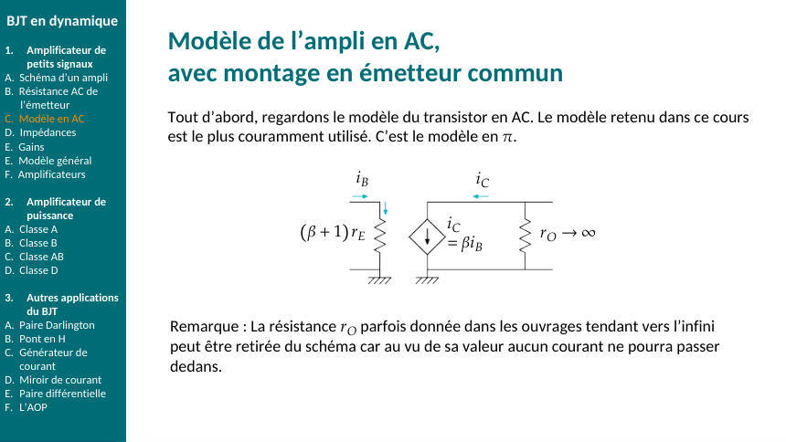
Schéma AC : \(C\) = fils, \(V_{\mathrm{CC}}\) = masse, \(R_{E}\) court-circuitée par \(C_{3}\)
Entrée : \(R_{1}\) et \(R_{2}\) tous deux entre base et masse (\(V_{\mathrm{CC}}\) est à la masse en AC) ⟹ en parallèle avec \((\beta +1)r_{E}\). Sortie : \(R_{C}\) entre collecteur et masse.
Gains et impédances
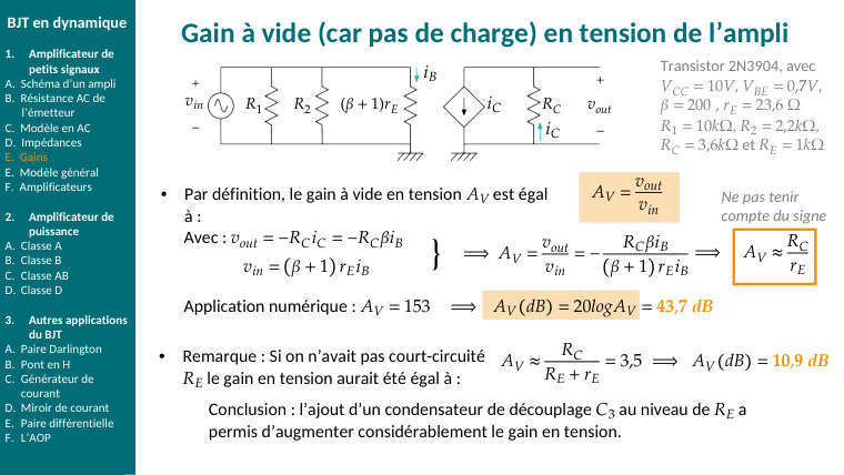
\(\displaystyle A_{V}=-R_{C}\,/\,r_{E}=-3300\,/\,39\approx -84\Longrightarrow 20\cdot \log (84)\approx 38{,}5\,\mathrm{d}B,\,\allowbreak \text{ déphasage }\,180\text{°}\) \(\displaystyle Z_{\mathrm{in}}=R_{1}//R_{2}//(\beta +1)\,r_{E}=1{,}8\,\mathrm{k}//(151\,\cdot \,39=5{,}9\,\mathrm{k})\approx 1{,}38\,\mathrm{k\Omega }\) \(\displaystyle Z_{\mathrm{out}}=R_{C}=3{,}3\,\mathrm{k\Omega }\)
Avec la charge \(R_{L}\) (diviseur de tension en sortie)
\(\displaystyle A_{V,\,\mathrm{charg}}\text{é }=A_{V}\,\cdot \,\frac{R_{L}}{Z_{\mathrm{out}}+R_{L}}=-84\,\cdot \,\frac{10}{13{,}3}\approx -63\,\left(\text{équivalent }\colon -\frac{R_{C}//R_{L}}{r_{E}}=-2{,}48\,\mathrm{k}/39\approx -63\right)\)
Sans \(C_{3}\)
\(\displaystyle A_{V}=-R_{C}\,/\,(R_{E}+r_{E})=-3300\,/\,2239\approx -1{,}5\)
Le découplage multiplie le gain par ~57. En échange, sans \(C_{3}\) le gain \(\approx \frac{-R_{C}}{R_{E}}\) est indépendant de \(r_{E}\), donc de la température : compromis gain / stabilité.

Réponse\(r_{E}\approx 39\,\mathrm{\Omega };\,\allowbreak A_{V}\approx -84\,(38{,}5\,\mathrm{d}B);\,\allowbreak Z_{\mathrm{in}}\approx 1{,}4\,\mathrm{k\Omega };\,\allowbreak Z_{\mathrm{out}}=3{,}3\,\mathrm{k\Omega }\) ; chargé \(\approx -63\) ; sans \(C_{3}\approx -1{,}5\).

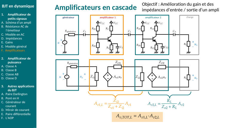
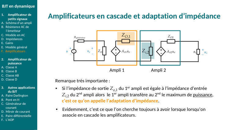
Le fil conducteurTout le chapitre 5 tient dans : \(Q\) (DC) \(\Longrightarrow r_{E}\Longrightarrow\) modèle en \(\pi \Longrightarrow\) trois nombres \((A_{V},\,\allowbreak Z_{\mathrm{in}},\,\allowbreak Z_{\mathrm{out}})\). Ensuite l'ampli est une boîte noire qu'on charge ou qu'on cascade avec des diviseurs de tension.

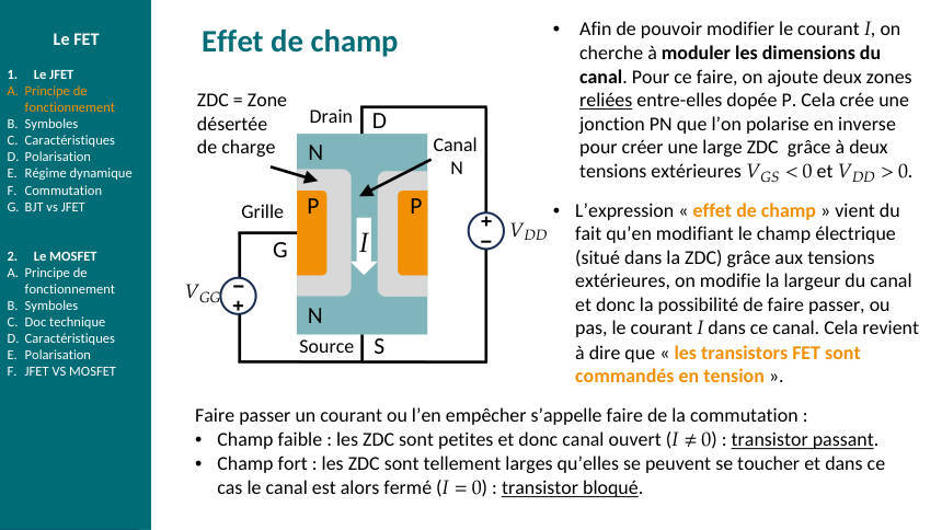
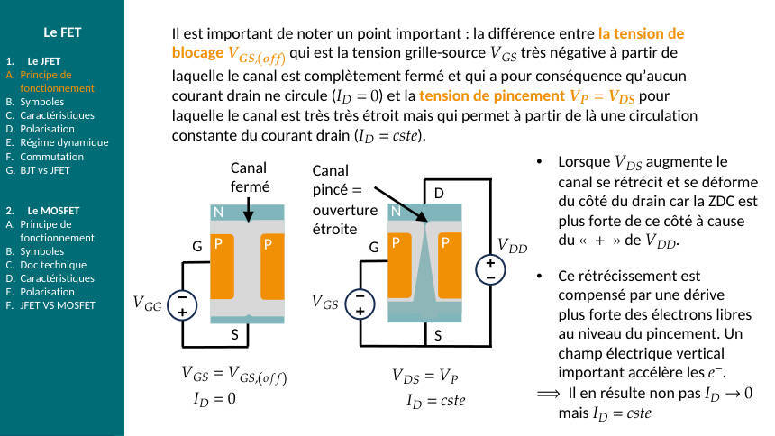
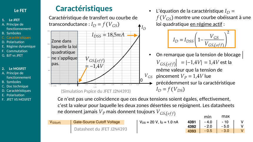
E11Ch. 6 · JFET autopolarisé

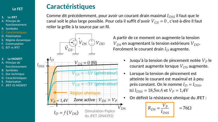
\(I_{\mathrm{DSS}}=10\,\mathrm{mA},\,\allowbreak V_{\mathrm{GS},\,\mathrm{off}}=-4\,\mathrm{V},\,\allowbreak R_{S}=500\,\mathrm{\Omega },\,\allowbreak R_{D}=1\,\mathrm{k\Omega },\,\allowbreak V_{\mathrm{DD}}=15\,\mathrm{V}\), grille à la masse par \(R_{G}\)

Ce qu'on chercheLe point de repos \((V_{\mathrm{GS}},\,\allowbreak I_{D},\,\allowbreak V_{\mathrm{DS}})\), la vérification de la zone active, puis \(g_{m}\) et le gain en source commune.

Équation de la maille grille-source
\(I_{G}=0\Longrightarrow V_{G}=0;\,\allowbreak V_{S}=R_{S}\,I_{D}\Longrightarrow\)
\(\displaystyle V_{\mathrm{GS}}=-R_{S}\,\cdot \,I_{D}=-0{,}5\,\cdot \,I_{D}\,(V\text{ en volts},\,\allowbreak I_{D}\text{ en }\,mA)\)
Injecter dans la loi quadratique
\(\displaystyle I_{D}=I_{\mathrm{DSS}}\,\left(1-\frac{V_{\mathrm{GS}}}{V_{\mathrm{GS},\,\mathrm{off}}}\right)^{2}=10\,\left(1-\frac{(-0{,}5\,I_{D})}{-4}\right)^{2}=10\,(1-0{,}125\,I_{D})^{2}\) \(\displaystyle I_{D}=10-2{,}5\,I_{D}+0{,}15625\,I_{D}^{2}\Longrightarrow 0{,}15625\,I_{D}^{2}-3{,}5\,I_{D}+10=0\)
Résoudre et choisir la racine
\(\displaystyle \Delta =3{,}5^{2}-4\,\cdot \,0{,}15625\,\cdot \,10=12{,}25-6{,}25=6\Longrightarrow \sqrt{\Delta }\approx 2{,}45\) \(\displaystyle I_{D}=\frac{(3{,}5\,\pm \,2{,}45)}{(2\,\cdot \,0{,}15625)}=\frac{(3{,}5\,\pm \,2{,}45)}{0{,}3125}\Longrightarrow 19{,}0\,\mathrm{mA}\text{ ou }\,3{,}36\,\mathrm{mA}\)
\(19\,\mathrm{mA}\gt I_{\mathrm{DSS}}\) et donnerait \(V_{\mathrm{GS}}=-9{,}5\,\mathrm{V}\lt V_{\mathrm{GS},\,\mathrm{off}}\) : impossible. On garde \(I_{D}=3{,}36\,\mathrm{mA}\), \(V_{\mathrm{GS}}=-1{,}68\,\mathrm{V}\) (bien entre −4 et 0 ✓).
\(V_{\mathrm{DS}}\) et zone de fonctionnement
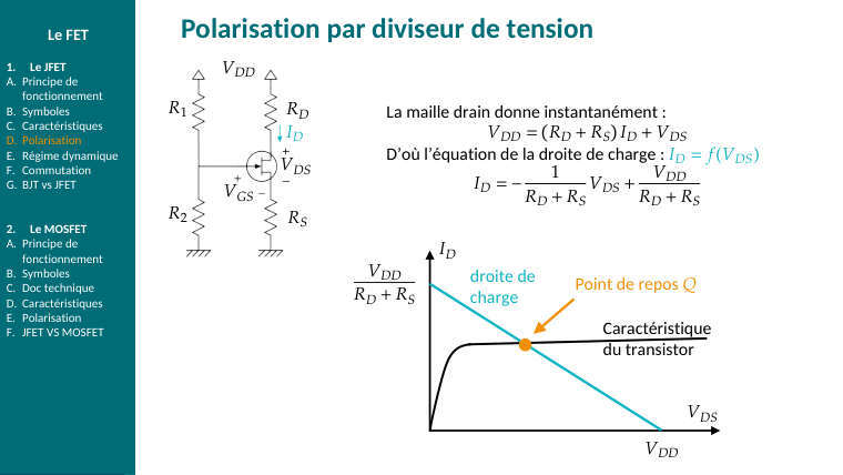
\(\displaystyle V_{\mathrm{DS}}=V_{\mathrm{DD}}-(R_{D}+R_{S})\,I_{D}=15-1{,}5\,\mathrm{k}\,\cdot \,3{,}36\,\mathrm{m}\approx 10\,\mathrm{V}\) \(\displaystyle \text{Condition zone active }\colon V_{\mathrm{DS}}\gt V_{\mathrm{GS}}-V_{\mathrm{GS},\,\mathrm{off}}=-1{,}68+4=2{,}3\,\mathrm{V}\Longrightarrow 10\gt 2{,}3\text{ ✓}\)
Transconductance et gain (source commune, \(R_{S}\) découplée)
\(\displaystyle g_{m}=(2\,I_{\mathrm{DSS}}/|V_{P}|)\left(1-\frac{V_{\mathrm{GS}}}{V_{\mathrm{GS},\,\mathrm{off}}}\right)=(20\,\mathrm{m}/4)(1-0{,}42)=5\,\mathrm{m}\,\cdot \,0{,}58\approx 2{,}9\,\mathrm{mS}\) \(\displaystyle A_{V}=-g_{m}\,R_{D}=-2{,}9\,\mathrm{m}\,\cdot \,1\,\mathrm{k}\approx -2{,}9\)
Faible gain : c'est la contrepartie de l'impédance d'entrée énorme du FET.

Réponse\(I_{D}\approx 3{,}4\,\mathrm{mA},\,\allowbreak V_{\mathrm{GS}}\approx -1{,}7\,\mathrm{V},\,\allowbreak V_{\mathrm{DS}}\approx 10\,\mathrm{V}\) (zone active) ; \(g_{m}\approx 2{,}9\,\mathrm{mS},\,\allowbreak A_{V}\approx -2{,}9\).

Sans calcul : la méthode graphiqueTracer la parabole \(I_{D}(V_{\mathrm{GS}})\) entre \(V_{\mathrm{GS},\,\mathrm{off}}\) et 0, et la droite \(V_{\mathrm{GS}}=-R_{S}I_{D}\) (passe par l'origine, pente \(\frac{-1}{R_{S}}\)). L'intersection est \(Q\). Utile pour vérifier l'ordre de grandeur de la racine choisie.

E12Ch. 6 · MOSFET

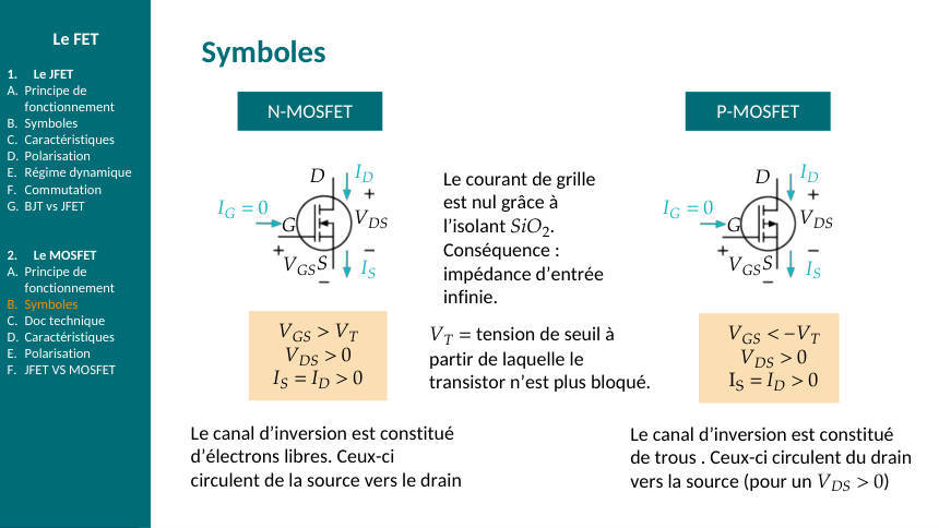
\(N\)-MOS avec \(K_{n}\cdot \frac{W}{L}=2\,\mathrm{mA}/\,\mathrm{V}^{2},\,\allowbreak V_{T}=1\,\mathrm{V},\,\allowbreak V_{\mathrm{GS}}=3\,\mathrm{V},\,\allowbreak V_{\mathrm{DD}}=10\,\mathrm{V}\). \((a)\,R_{D}=1{,}5\,\mathrm{k\Omega };\,\allowbreak (b)\,R_{D}=5\,\mathrm{k\Omega }\).

Ce qu'on chercheLa région de fonctionnement et \(I_{D},\,\allowbreak V_{\mathrm{DS}},\,\allowbreak g_{m}\). Méthode : supposer saturé, vérifier \(V_{\mathrm{DS}}\ge V_{\mathrm{GS}}-V_{T}\).

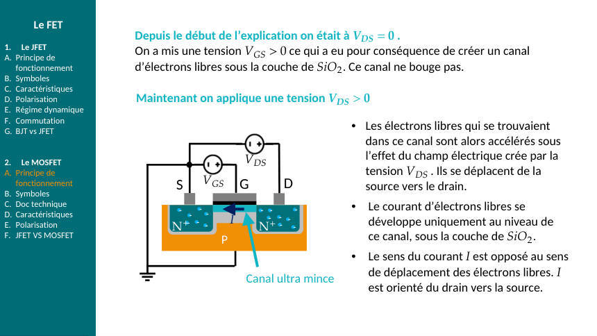
Le transistor conduit-il ?
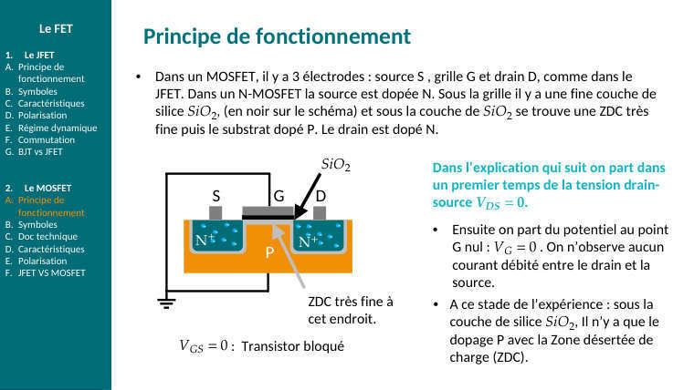
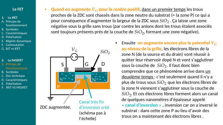
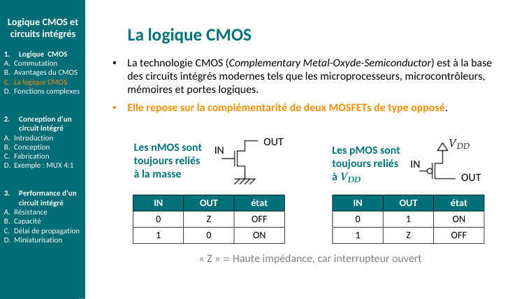
\(V_{\mathrm{GS}}=3\,\mathrm{V}\gt V_{T}=1\,\mathrm{V}\Longrightarrow\) canal d'inversion formé ⟹ conduit. Tension de commande utile : \(V_{\mathrm{GS}}-V_{T}=2\,\mathrm{V}\).
Hypothèse « saturé » (zone active)
\(\displaystyle I_{D}=\frac{1}{2}\,\cdot \,K_{n}\,\left(\frac{W}{L}\right)\,\cdot \,(V_{\mathrm{GS}}-V_{T})^{2}=\frac{1}{2}\,\cdot \,2\,\mathrm{m}\,\cdot \,2^{2}=4\,\mathrm{mA}\)
\((a)\,R_{D}=1{,}5\,\mathrm{k\Omega }\) — vérification
\(\displaystyle V_{\mathrm{DS}}=V_{\mathrm{DD}}-R_{D}\,I_{D}=10-1{,}5\,\mathrm{k}\,\cdot \,4\,\mathrm{m}=4\,\mathrm{V}\ge V_{\mathrm{GS}}-V_{T}=2\,\mathrm{V}\text{ ✓ saturé confirmé}\) \(\displaystyle g_{m}=2\,\frac{I_{D}}{V_{\mathrm{GS}}-V_{T}}=8\,\mathrm{m}\,/\,2=4\,\mathrm{mS}\)
\((b)\,R_{D}=5\,\mathrm{k\Omega }\) — vérification
\(\displaystyle V_{\mathrm{DS}}=10-5\,\mathrm{k}\,\cdot \,4\,\mathrm{m}=-10\,\mathrm{V}\Longrightarrow \text{ absurde }\,(V_{\mathrm{DS}}\lt 0)\)
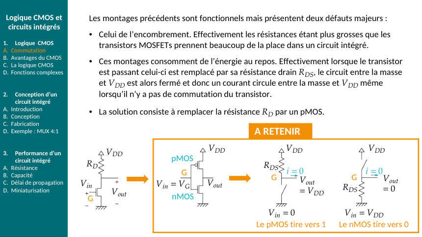
L'hypothèse est fausse : le transistor est en région ohmique (canal non pincé). \(I_{D}\) est plus petit que \(4\,\mathrm{mA}\) et \(V_{\mathrm{DS}}\) est petit ; il se comporte comme une résistance \(R_{\mathrm{DS}}\approx \frac{1}{K_{n}\left(\frac{W}{L}\right)(V_{\mathrm{GS}}-V_{T})}=250\,\mathrm{\Omega }\), d'où \(V_{\mathrm{DS}}\approx 10\,\cdot \,\frac{250}{5250}\approx 0{,}5\,\mathrm{V}\). C'est le régime « interrupteur fermé » du chapitre 7.

Réponse(a) saturé : \(I_{D}=4\,\mathrm{mA},\,\allowbreak V_{\mathrm{DS}}=4\,\mathrm{V},\,\allowbreak g_{m}=4\,\mathrm{mS}\). \((b)\) ohmique : \(V_{\mathrm{DS}}\approx 0{,}5\,\mathrm{V}\), le MOS agit en interrupteur fermé.

Trois régions, un seul test\(V_{\mathrm{GS}}\lt V_{T}\) : bloqué. Sinon, \(V_{\mathrm{DS}}\ge V_{\mathrm{GS}}-V_{T}\) : saturé (source de courant, pour amplifier). \(V_{\mathrm{DS}}\lt V_{\mathrm{GS}}-V_{T}\) : ohmique (résistance commandée, pour commuter). Le MOSFET logique (ch. 7) vit dans bloqué/ohmique, jamais en saturé.

E13Ch. 7 · Synthèse CMOS

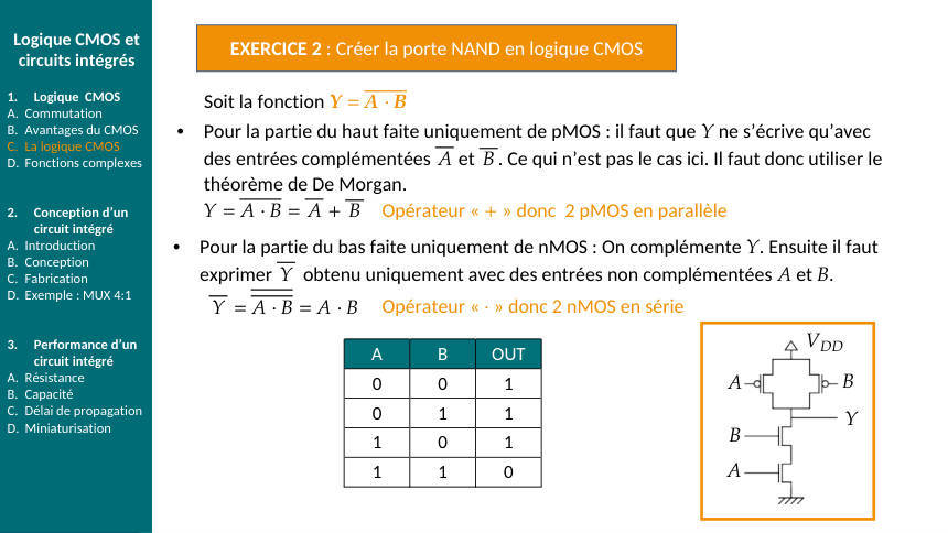
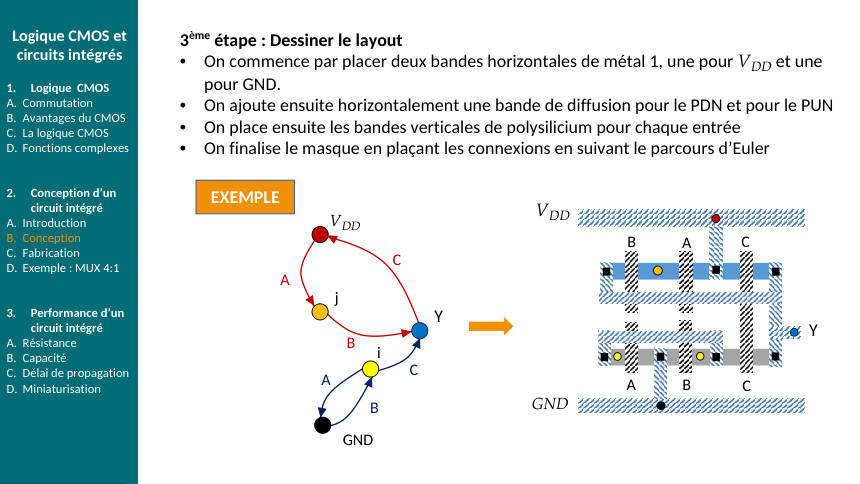
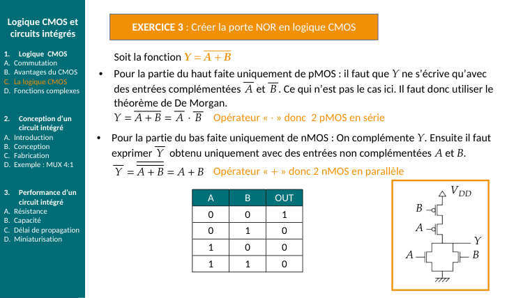
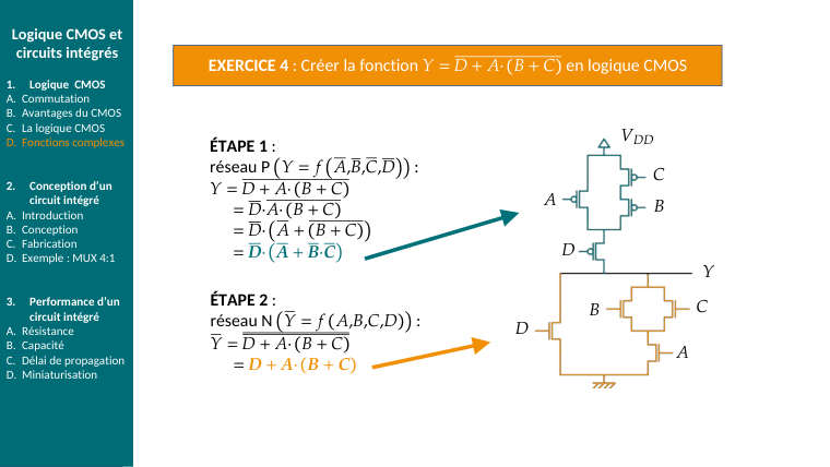
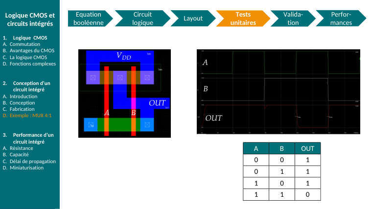
Réaliser \(Y\) = \(A\cdot B+C\) en logique CMOS et compter les transistors

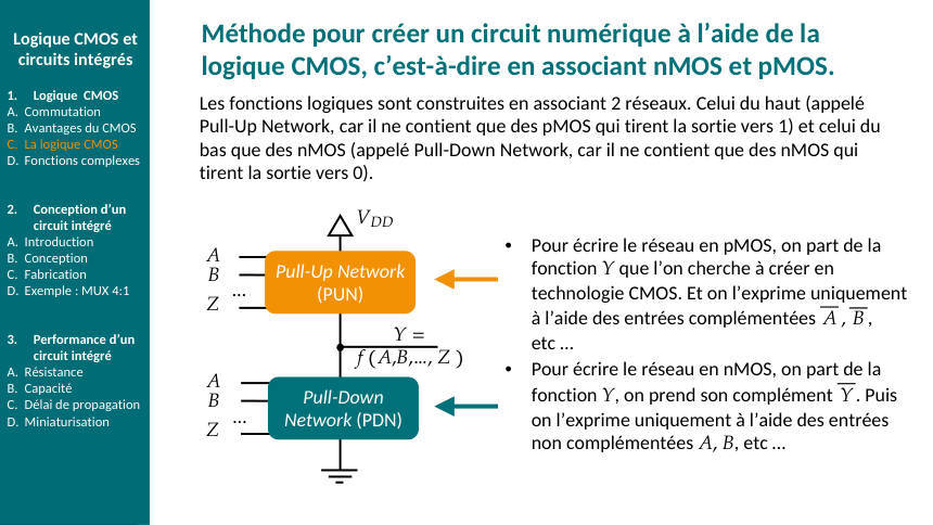
Ce qu'on chercheLe réseau PDN (nMOS, vers GND) et le réseau PUN (pMOS, vers \(V_{\mathrm{DD}}\)), puis la vérification sur la table de vérité.

PDN : partir de \(\bar{Y}\), entrées non complémentées
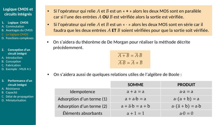
\(\displaystyle \bar{Y}=A\cdot B+C\Longrightarrow \text{ « }\,\cdot \text{ » }=\text{ série},\,\allowbreak \text{ « }+\text{ » }=\text{ parallèle}\) \(\displaystyle PDN=(\text{nMOS}_{A}\text{ en série avec nMOS}_{B})\text{ en parallèle avec nMOS}_{C}\)
Lecture : la sortie est tirée à 0 si (\(A\) et \(B\)) ou si \(C\).
PUN : la structure duale (série ↔ parallèle), mêmes entrées, transistors pMOS
\(\displaystyle Y=\overline{(A\cdot B+C)}=\overline{(A\cdot B)}\,\cdot \,\bar{C}=(\bar{A}+\bar{B})\,\cdot \,\bar{C}\,(\text{De Morgan deux fois})\) \(\displaystyle PUN=(\text{pMOS}_{A}\text{ en parallèle avec pMOS}_{B})\text{ en série avec pMOS}_{C}\)
Un pMOS conduit quand son entrée vaut 0 : la sortie est tirée à 1 si (\(A=0\) ou \(B=0\)) et \(C=0\). ✓ cohérent avec \(Y\).
Compter
3 entrées \(\Longrightarrow 3\) nMOS + 3 pMOS = 6 transistors. Règle : une fonction à \(n\) entrées réalisée en une seule porte complexe (AOI) coûte \(2\,\mathrm{n}\) transistors.
Vérifier une ligne de la table
\(A=1,\,\allowbreak B=1,\,\allowbreak C=0\) : PDN : \(A\cdot B\) conduit ⟹ chemin vers GND \(\Longrightarrow Y=0\). PUN : pMOS_A et pMOS_B tous deux ouverts ⟹ pas de chemin vers \(V_{\mathrm{DD}}\) ✓ (jamais les deux réseaux fermés en même temps : pas de court-circuit).

RéponsePDN : (\(A\) série \(B\)) // \(C\) ; PUN : \((A//B)\) série \(C;\,\allowbreak 6\) transistors.

Si la fonction n'est pas « inversée »\(Y=A\cdot B+C\) (sans barre) n'est pas réalisable en une seule porte CMOS (une porte CMOS statique est toujours inverseuse). On réalise \(A\cdot B+C\) \((6\,\mathrm{T})\) puis un inverseur \((2\,\mathrm{T})=8\) transistors. Même logique pour AND = NAND + NOT.

E14Ch. 7 · Résistances, capacités, délai

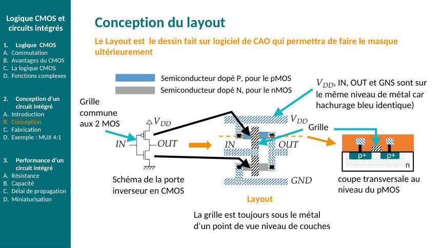
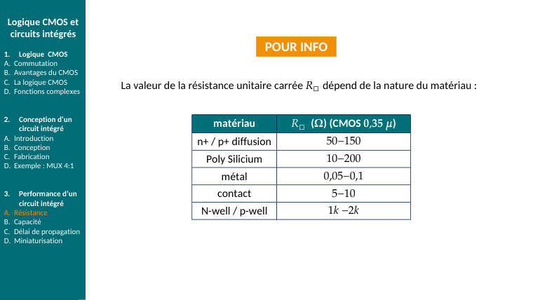
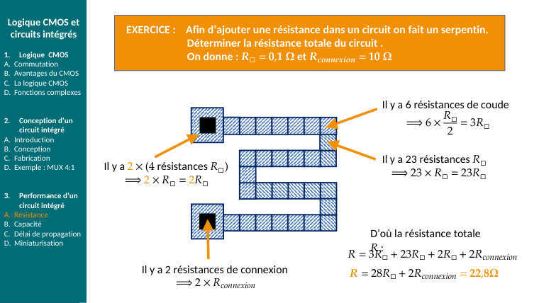
\(R_{\square }\)(métal) \(=0{,}1\,\mathrm{\Omega }\), rail de \(40\,\lambda \,\times \,4\,\lambda\) avec un coude ; \(R_{N}=R_{P}=5\,\mathrm{k\Omega };\,\allowbreak C_{\mathrm{OUT}}=20\,\mathrm{fF}\). Délai d'un inverseur, puis d'une NAND3.

Ce qu'on chercheAppliquer la méthode des carrés, puis le modèle RC du délai, puis la règle du carré du nombre de transistors en série.

Résistance du rail par comptage de carrés
\(\displaystyle \text{nombre de carrés }=\frac{\ell }{w}=\frac{40}{4}=10;\,\allowbreak \text{ un coude compte }\,\frac{1}{2}\text{ carré}\) \(\displaystyle R_{\mathrm{rail}}=R_{\square }\,\cdot \,(10+0{,}5)=0{,}1\,\cdot \,10{,}5\approx 1{,}05\,\mathrm{\Omega }\)
Négligeable devant les \(5\,\mathrm{k\Omega }\) des transistors : c'est en général le cas pour le métal, pas pour le polysilicium (\(R_{\square }\) ~ \(10-50\,\mathrm{\Omega }\)).
Délai de l'inverseur
\(\displaystyle \tau =(R_{N}+R_{P})\,\cdot \,C_{\mathrm{OUT}}\,/\,2=(5\,\mathrm{k}+5\,\mathrm{k})\,\cdot \,20\,f\,/\,2=100\,\mathrm{ps}\)
NAND à 3 entrées : 3 nMOS en série dans le PDN
\(\displaystyle \tau _{\mathrm{descente}}\approx \left(\frac{n^{2}}{2}\right)\,\cdot \,R_{N}\,\cdot \,C=\left(\frac{9}{2}\right)\,\cdot \,5\,\mathrm{k}\,\cdot \,20\,f=450\,\mathrm{ps}\,(\text{Elmore})\) \(\displaystyle \tau _{\mathrm{mont}}ée\colon \text{ les }\,3\text{ pMOS sont en parallèle }\Longrightarrow \text{ au pire un seul conduit }\colon R_{P}\,\cdot \,C=100\,\mathrm{ps}\)
Le délai « pire cas » est \(450\,\mathrm{ps}\) : la NAND3 est ~4,5 fois plus lente que l'inverseur sur le front descendant.
Fréquence \(\max\) et miniaturisation
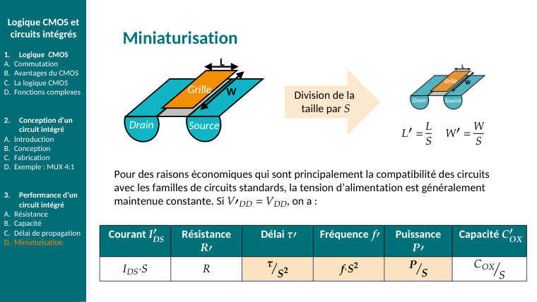
Chaîne de 5 portes de \(100\,\mathrm{ps}\) : chemin critique \(0{,}5\,\mathrm{ns}\Longrightarrow\) période \(\ge 1\,\mathrm{ns}\Longrightarrow f\lt 1\,\mathrm{GHz}\). En divisant les dimensions par \(S=2\) (\(V_{\mathrm{DD}}\) constant) : \(\tau \to \frac{\tau }{4},\,\allowbreak f\to 4f\).

Réponse\(R_{\mathrm{rail}}\approx 1\,\mathrm{\Omega };\,\allowbreak \tau _{\mathrm{inv}}=100\,\mathrm{ps};\,\allowbreak \tau _{\mathrm{NAND3}}\approx 450\,\mathrm{ps}\) (descente) / \(100\,\mathrm{ps}\) (montée).

Pourquoi \(n^{2}\) et pas \(n\)\(n\) transistors en série : la résistance totale est \(nR\) et chaque nœud intermédiaire porte sa capacité ; la somme des produits \(R\times C\) cumulés donne \(\approx \frac{n^{2}}{2}\). Conséquence de conception : on évite plus de 3–4 transistors en série et on met les entrées « tardives » près de la sortie.

🧰 À connaître à côté

Ce qui n'est pas « au programme » mais qui fait la différence

Ordres de grandeur, calcul mental des parallèles et des dB, unités, constantes du silicium, lecture d'une datasheet, résolution d'un second degré… et les pièges classiques par chapitre. À relire la veille.

📎 Le kit de calcul

// Résistances en parallèle, de tête

Formule : \(R_{1}//R_{2}=\frac{R_{1}R_{2}}{R_{1}+R_{2}}\). Deux résistances égales \(\Longrightarrow \frac{R}{2}\). Trois égales \(\Longrightarrow \frac{R}{3}\).
Rapport \(\ge 10\) : \(R_{1}//R_{2}\approx \text{ la plus petite}\) (à 10 % près). \(100\,\mathrm{k}//1\,\mathrm{k}\approx 0{,}99\,k\).
Le résultat est toujours inférieur à la plus petite des deux. Sinon, erreur.
Série : les tensions s'ajoutent (diviseur de tension). Parallèle : les courants s'ajoutent (diviseur de courant).
Astuce \(mA\cdot k\,\mathrm{\Omega }\colon 4{,}3\,\mathrm{mA}\,\times \,1\,\mathrm{k\Omega }=4{,}3\,\mathrm{V};\,\allowbreak 43\,\mu A\,\times \,100\,\mathrm{k\Omega }=4{,}3\,\mathrm{V}\).

dB Décibels sans calculatrice

Gain	\(20\cdot \log\) (tension)	Gain	\(20\cdot \log\)
\(\times 1\)	\(0\,\mathrm{d}B\)	\(\times 0{,}5\)	\(-6\,\mathrm{d}B\)
\(\times \sqrt{2}\approx 1{,}41\)	\(3\,\mathrm{d}B\)	\(\times 0{,}707\)	\(-3\,\mathrm{d}B\)
\(\times 2\)	\(6\,\mathrm{d}B\)	\(\times 5\)	\(14\,\mathrm{d}B\)
\(\times 10\)	\(20\,\mathrm{d}B\)	\(\times 100\)	\(40\,\mathrm{d}B\)
\(\times 20\)	\(26\,\mathrm{d}B\)	\(\times 1000\)	\(60\,\mathrm{d}B\)

Les gains se multiplient, les dB s'ajoutent : \(84=10\,\times \,8{,}4\Longrightarrow 20+18{,}5=38{,}5\,\mathrm{d}B\). Puissance : \(10\cdot \log (\times 2=3\,\mathrm{d}B,\,\allowbreak \times 10=10\,\mathrm{d}B)\).

Si Constantes du silicium à \(300\,\mathrm{K}\)

\(n_{i}\approx 1{,}5\cdot 10^{10}\,\mathrm{cm}^{-3}\) (parfois \(1{,}0\cdot 10^{10}\) selon la source — prendre celle de l'énoncé)
\(E_{g}\approx 1{,}12\,\mathrm{eV}\) ; densité atomique \(\approx 5\cdot 10^{22}\,\mathrm{cm}^{-3}\)
\(\mu _{n}\approx 1350,\,\allowbreak \mu _{p}\approx 480\,\mathrm{cm}^{2}/V\cdot s\,(\mu _{n}\approx 3\,\mu _{p})\)
\(\frac{k_{B}T}{e}=26\,\mathrm{mV};\,\allowbreak \frac{D}{\mu }=26\,\mathrm{mV}\) (Einstein)
\(V_{S}\approx 0{,}7\,\mathrm{V}\) (Si), \(0,\,\allowbreak 3\,\mathrm{V}\) (Ge), \(0,\,\allowbreak 2-0{,}4\,\mathrm{V}\) (Schottky), \(1,\,\allowbreak 8-3{,}3\,\mathrm{V}\) (LED selon couleur)
\(I_{S}\) double tous les \(\approx 10^{\circ}\mathrm{C};\,\allowbreak V_{D}\) baisse de \(\approx 2\,\mathrm{mV}/^{\circ}\mathrm{C}\) à \(I\) constant

\(1\,\mathrm{eV}=1{,}6\cdot 10^{-19}\,\mathrm{J}\). \(1\,\mathrm{S}/cm=100\,\mathrm{S}/\,\mathrm{m}\). \(1\,\mathrm{cm}^{-3}=10^{6}\,\mathrm{m}^{-3}\).

\(10^{n}\) Préfixes et unités

\(p\)	\(n\)	\(\mu\)	\(m\)	\(k\)	\(M\)	\(G\)
\(10^{-12}\)	\(10^{-9}\)	\(10^{-6}\)	\(10^{-3}\)	\(10^{3}\)	\(10^{6}\)	\(10^{9}\)

\(\Omega =\frac{V}{A};\,\allowbreak S=\frac{A}{V}=\frac{1}{\Omega };\,\allowbreak F=\frac{C}{V}=A\cdot \frac{s}{V};\,\allowbreak H=V\cdot \frac{s}{A}\).
\(\gamma\) en \(\frac{S}{m};\,\allowbreak \rho\) en \(\Omega \cdot m;\,\allowbreak j\) en \(\frac{A}{m^{2}};\,\allowbreak E\) en \(\frac{V}{m};\,\allowbreak \mu\) en \(\frac{m^{2}}{V\cdot s}\).
\(g_{m}\) en \(S\) (\(mS\) typiquement) ; \(r_{E}\) en \(\Omega ;\,\allowbreak \tau =RC\) en \(s\) (\(k\,\mathrm{\Omega }\,\times \,pF\) = ns, \(k\,\mathrm{\Omega }\,\times \,fF\) = ps).
Puissance : \(P=U\cdot I=R\cdot I^{2}=\frac{U^{2}}{R}\). Une résistance \(\frac{1}{4}\,W\) supporte \(\approx 15\,\mathrm{mA}\) sous \(15\,\mathrm{V}\,(P=0{,}22\,\mathrm{W})\).

\(x^{2}\) Second degré et logarithmes

\(ax^{2}+bx+c=0\Longrightarrow \Delta =b^{2}-4ac,\,\allowbreak x=\frac{(-b\,\pm \,\sqrt{\Delta })}{2a}\). En électronique, une seule racine est physique : vérifier \(V_{\mathrm{GS},\,\mathrm{off}}\lt V_{\mathrm{GS}}\lt 0,\,\allowbreak I_{D}\lt I_{\mathrm{DSS}},\,\allowbreak V_{\mathrm{DS}}\gt 0\).
\(\ln (a\cdot 10\text{ᵏ})=\ln \,a+2{,}3\,\mathrm{k}\) ; \(\ln \,2=0{,}69,\,\allowbreak \ln \,3=1{,}10,\,\allowbreak \ln \,5=1{,}61,\,\allowbreak \ln \,10=2{,}30\).
\(e^{x}\) : \(e^{\frac{0{,}7}{0{,}026}}=e^{27}\approx 5\cdot 10^{11}\) — d'où le « mur » de la caractéristique de diode à \(0{,}7\,\mathrm{V}\).
Shockley inversé : \(V_{D}=\eta V_{T}\,\cdot \,\ln \left(\frac{I_{D}}{I_{S}}+1\right)\). \(\times 10\) sur \(I_{D}\Longrightarrow +60\,\mathrm{mV}\) sur \(V_{D}\,(\eta =1)\).

📄 Lire une datasheet

Absolute maximum ratings : à ne jamais dépasser \((V_{\mathrm{CEO}},\,\allowbreak I_{C,\,\mathrm{max}},\,\allowbreak P_{\mathrm{tot}},\,\allowbreak V_{\mathrm{RRM}})\). Ce ne sont pas des valeurs de fonctionnement.
\(h_{\mathrm{FE}}\) \(=\beta\), donné en plage (ex. 100–300) à un \(I_{C}\) et \(V_{\mathrm{CE}}\) précis. Prendre le \(\min\) pour dimensionner une saturation, le typique pour un ampli.
\(V_{\text{CE}(\text{sat})}\) donné pour un couple \((I_{C},\,\allowbreak I_{B})\), souvent \(\frac{I_{C}}{I_{B}}=10\).
\(V_{\text{BE}(\text{on})}\) \(\approx 0{,}65-0{,}7\,\mathrm{V}\) ; \(V_{\text{GS}(\text{th})}\) \(=V_{T}\,\mathrm{d}u\) MOSFET, en plage aussi.
\(I_{\mathrm{DSS}},\,\allowbreak V_{\text{GS}(\text{off})}\) pour un JFET : très dispersés (facteur 2–3 d'un exemplaire à l'autre) — d'où l'intérêt de l'autopolarisation.
Les courbes sont à \(25^{\circ}\mathrm{C}\) sauf mention. \(\beta\) et \(I_{S}\) montent avec \(T\).

✏ Conventions et notations

Majuscules = grandeurs DC / totales \((I_{C},\,\allowbreak V_{\mathrm{CE}})\) ; minuscules = petites variations AC \((i_{c},\,\allowbreak v_{\mathrm{ce}})\). Total = DC + AC.
Indice double \(V_{\mathrm{CE}}=V_{C}-V_{E}\). Indice répété \(V_{\mathrm{CC}},\,\allowbreak V_{\mathrm{DD}}\) = alimentation.
Convention récepteur : flèche de tension et flèche de courant en sens opposés \(\Longrightarrow u\) = Ri. Générateur : même sens.
NPN : flèche de l'émetteur vers l'extérieur (« Not Pointing \(iN\) »). PNP : vers l'intérieur. Courants : \(I_{E}\) sort du NPN.
Masse = référence \(0\,\mathrm{V}\), tous les potentiels s'y rapportent. Un nœud à \(V_{\mathrm{CC}}\) est « à la masse » en AC.

🧠 Ordres de grandeur « radar »

Grandeur	Plausible	Suspect
\(I_{B}\)	\(1-100\,\mu A\)	\(\gt 1\,\mathrm{mA}\)
\(I_{C},\,\allowbreak I_{D}\)	\(0{,}1-50\,\mathrm{mA}\)	\(\gt 1\,\mathrm{A}\,(\text{sauf puissance})\)
\(r_{E}\)	\(5-100\,\mathrm{\Omega }\)	\(k\,\mathrm{\Omega }\)
\(\|A_{V}\|\) émetteur commun	\(20-300\)	\(\gt 1000\)
\(Z_{\mathrm{in}}\) BJT / \(FET\)	\(k\,\mathrm{\Omega }\,/\,M\,\mathrm{\Omega }\)	\(\Omega\)
\(V_{0}\) jonction Si	\(0{,}6-0{,}9\,\mathrm{V}\)	\(\gt 1{,}2\,\mathrm{V}\)
\(\tau\) porte CMOS	\(10\,\mathrm{ps}-1\,\mathrm{ns}\)	\(\mu s\)
\(V_{\mathrm{CE}}\) en mode actif	\(1\,\mathrm{V}\ldots V_{\mathrm{CC}}-1\,\mathrm{V}\)	\(\lt 0\text{ ou }\gt V_{\mathrm{CC}}\)

🔭 Hors programme, mais attendu d'un ingénieur ECE

Ce que le cours ne détaille pas et que les TP, les projets et la suite du cursus supposent acquis. Le poly annonce aussi deux cours sans exercices (PCB et mémoires) : l'essentiel est résumé ici.

🔢 Valeurs normalisées \(E_{12}\,/\,E_{24}\)

On n'achète pas une résistance de \(266{,}7\,\mathrm{\Omega }\) : on choisit la valeur normalisée la plus proche, dans une série à 12 ou 24 valeurs par décade.

\(\displaystyle E_{12}\,(\pm 10\%)\colon 10\,12\,15\,18\,22\,27\,33\,39\,47\,56\,68\,82\) \(\displaystyle E_{24}\,(\pm 5\%)\colon 10\,11\,12\,13\,15\,16\,18\,20\,22\,24\,27\,30\) \(\displaystyle 33\,36\,39\,43\,47\,51\,56\,62\,68\,75\,82\,91\)

Condensateurs courants : \(1\,\cdot \,2{,}2\,\cdot \,4{,}7\,(\times 10^{n})\). Après avoir choisi, recalculer le point de fonctionnement avec la valeur retenue et vérifier que le cahier des charges tient avec la tolérance.

🧪 Simuler avant de souder

LTspice (gratuit, Analog Devices) : SPICE complet, modèles de vrais composants (1N4148, 2N2222, 2N3904…). Analyses .op (point de repos), .tran (temporel), .ac (Bode).
Falstad / CircuitJS (dans le navigateur) : animation des courants, parfait pour « voir » un redresseur ou un régulateur Zener.
KiCad (libre) : schéma, simulation ngspice et routage de PCB.

Réflexe : refaire un exercice de TD en simulation et comparer au calcul à la main. Un écart de plus de 10 % signale une hypothèse fausse (état d'une diode, régime du transistor).

🟩 Le PCB en bref (cours 6 du poly)

Couches : cuivre (1 à \(n\) couches) sur époxy FR-4 ; vernis épargne (vert) ; sérigraphie (textes).
Pistes : largeur selon le courant (ordre de grandeur : \(0{,}3\,\mathrm{mm}\) pour ~\(1\,\mathrm{A}\) en cuivre de \(35\,\mu m\), à vérifier avec un calculateur IPC-2221) ; les plus courtes possible pour les signaux rapides.
Vias : trous métallisés qui relient les couches.
Plan de masse et découplage : un condensateur de \(100\,\mathrm{nF}\) au plus près de chaque broche d'alimentation de CI.
Composants traversants (THT) ou montés en surface \(\left(\frac{CMS}{SMD}\right)\), voir chapitre 1.

💾 Les mémoires en bref (cours 9 du poly)

Type	Cellule	Volatile ?	Usage
SRAM	\(6\text{ transistors }\,(2\text{ inverseurs rebouclés }+2\text{ d'accès})\)	oui	caches du processeur
DRAM	\(1\text{ transistor }+1\text{ condensateur}\)	oui, à rafraîchir	mémoire vive
Flash	\(\text{MOS à grille flottante}\)	non	SSD, clés USB, microcontrôleurs
ROM	\(\text{câblée à la fabrication}\)	non	code figé

Plus une mémoire est rapide, plus elle est chère par bit : d'où la hiérarchie registres → caches SRAM → DRAM → Flash/disque. Les ions lourds peuvent faire basculer une SRAM (SEU) : voir l'exercice 11.5.

🔬 Mesurer en TP sans se tromper

Voltmètre en parallèle, ampèremètre en série (et jamais un ampèremètre directement sur une alimentation).
Oscilloscope : toutes les masses des voies sont reliées à la terre ; brancher une masse ailleurs qu'à la masse du circuit crée un court-circuit. Sonde \(\times 10\) pour les signaux rapides.
Couplage DC pour voir la composante continue (point de repos), AC pour zoomer sur un petit signal.
Mesurer un gain : amplitude crête à crête en sortie / en entrée ; vérifier qu'il n'y a pas d'écrêtage (sinon le transistor sature ou se bloque).

⚠ Les pièges classiques, chapitre par chapitre

Ch. 0 · diviseurUtiliser \(V_{2}=V\cdot \frac{R_{2}}{R_{1}+R_{2}}\) alors qu'une charge est branchée sur \(R_{2}\). ✓ Remplacer \(R_{2}\) par \(R_{2}//R_{L}\), ou passer par Thévenin.

Ch. 0 · ThéveninCalculer \(R_{\mathrm{Th}}\) en laissant les sources. ✓ Sources de tension → fil, sources de courant → trou, puis résistance vue des bornes.

Ch. 0 · AOPÉcrire \(V_{+}=V_{-}\) sans contre-réaction, ou oublier la saturation. ✓ Vérifier d'abord qu'une résistance relie la sortie à l'entrée −. Puis vérifier \(|V_{\mathrm{out}}|\lt V_{\mathrm{sat}}\).

Ch. 1 · section\(S=\pi d^{2}\) au lieu de \(\pi r^{2}=\frac{\pi d^{2}}{4}\) (facteur 4 sur \(R\)). ✓ Convertir le diamètre en rayon avant tout.

Ch. 1 · températureConclure « \(R\) augmente avec \(T\) » pour un semi-conducteur. ✓ Conducteur : \(R\nearrow\). Semi-conducteur et isolant : \(R\searrow\) (plus de porteurs).

Ch. 2 · minoritairesPrendre \(p=n_{i}\) dans un type \(N\). ✓ \(p=\frac{n_{i}^{2}}{N_{D}}\), bien plus petit que \(n_{i}\).

Ch. 2 · polarisationInverser le sens : « \(P\) au − = directe ». ✓ Directe \(=P\) au \(+,\,\allowbreak N\) au − (\(P\) comme Plus). La barrière \(V_{0}\) diminue.

Ch. 3 · état de la diodeDécider « passante » parce que la source est positive, sans vérifier \(E\gt V_{S}\). ✓ Hypothèse bloquée \(\to V_{D}\to\) comparer à \(0{,}7\,\mathrm{V}\).

Ch. 3 · ZenerOublier que la Zener doit être en inverse, ou oublier la résistance série. ✓ Cathode côté +. Sans \(R\) série, \(I_{Z}\) n'est pas limité : destruction.

Ch. 3 · GraëtzChute de \(V_{S}\) au lieu de \(2\,\mathrm{V}_{S}\). ✓ À chaque alternance, le courant traverse deux diodes en série.

Ch. 4 · saturationGarder \(I_{C}=\beta I_{B}\) alors que \(V_{\mathrm{CE}}\) calculé est négatif. ✓ \(I_{C}\le I_{C,\,\mathrm{sat}}=\frac{V_{\mathrm{CC}}}{R_{C}}\). Plafonner et prendre \(V_{\mathrm{CE},\,\mathrm{sat}}\).

Ch. 4 · pont diviseurCalculer \(V_{B}\) par le diviseur nu puis oublier \(R_{E}\) dans la maille. ✓ \(V_{E}=V_{B}-0{,}7\) puis \(I_{E}=\frac{V_{E}}{R_{E}}\). Et \(V_{\mathrm{CE}}=V_{\mathrm{CC}}-R_{C}I_{C}-R_{E}I_{E}\).

Ch. 5 · schéma ACLaisser \(V_{\mathrm{CC}}\) comme un nœud à part, ou laisser \(R_{E}\) alors que \(C_{3}\) la découple. ✓ \(V_{\mathrm{CC}}\to\) masse (\(R_{1}\) et \(R_{C}\) vont à la masse). \(C_{3}\) court-circuite \(R_{E}\).

Ch. \(5\,\cdot \,r_{E}\)Utiliser \(I_{C}\) en \(mA\) sans convertir : \(r_{E}=\frac{26}{4{,}3}\approx 6\,\mathrm{\Omega }\) est juste si 26 est en \(mV\) et \(I\) en \(mA\). ✓ Toujours \(26\,\mathrm{mV}\,/\,I_{E}(mA)=\Omega\).

Ch. 5 · dBÉcrire un gain négatif « −38 dB » pour \(A_{V}=-84\). ✓ \(\mathrm{d}B=20\cdot \log |A_{V}|=+38{,}5\,\mathrm{d}B\) ; le signe est un déphasage de \(\pi\).

Ch. 6 · racineGarder la racine \(I_{D}\gt I_{\mathrm{DSS}}\,\mathrm{d}u\) second degré. ✓ Contraintes physiques : \(0\lt I_{D}\lt I_{\mathrm{DSS}}\) et \(V_{\mathrm{GS},\,\mathrm{off}}\lt V_{\mathrm{GS}}\lt 0\) (JFET canal \(N\)).

Ch. \(6\,\cdot \,V_{P}\,vs\,V_{\mathrm{GS},\,\mathrm{off}}\)Les confondre dans les formules. ✓ Même valeur absolue ; \(V_{\mathrm{GS},\,\mathrm{off}}\lt 0\) dans la loi quadratique, \(V_{P}\gt 0\) dans \(R_{\mathrm{DS}}=\frac{V_{P}}{I_{\mathrm{DSS}}}\).

Ch. 7 · PUNMettre le même schéma en haut et en bas. ✓ \(PUN\) = dual du PDN : série ↔ parallèle. Et une porte CMOS est toujours inverseuse.

Ch. 7 · délaiMultiplier par \(n\) au lieu de \(\frac{n^{2}}{2}\) pour \(n\) transistors en série. ✓ Elmore : \(\approx \left(\frac{n^{2}}{2}\right)\)RC. C'est pourquoi on limite à 3–4 en série.

Ch. 3 · état d'une diodeConclure qu'une Zener conduit parce que \(E\gt V_{Z}\). ✓ Comparer \(V_{Z}\) à la tension à vide à ses bornes (Thévenin) : avec une charge faible, elle peut rester bloquée.

Ch. 4 · PNPFaire entrer le courant de base dans un PNP. ✓ Pour un PNP, \(I_{E}\) entre dans l'émetteur, \(I_{B}\) et \(I_{C}\) sortent.

Ch. 5 · condensateursDimensionner un découplage avec \(R_{1}+R_{2}\). ✓ Prendre la résistance vue par le condensateur (souvent un parallèle), et une coupure une décade sous \(f_{\mathrm{min}}\).

Ch. \(6\,\cdot \,K_{n}\)Utiliser \(g_{m}=2\,\mathrm{K}_{n}V_{ov}\) avec une loi en \(\frac{1}{2}K_{n}\). ✓ Recopier la loi de l'énoncé, puis dériver : \(g_{m}=\frac{\mathrm{d}I_{D}}{\mathrm{d}V_{\mathrm{GS}}}\).

Ch. 7 · MUXÉcrire \(s=\bar{z}x\) + zy sans vérifier quelle porte de transmission conduit. ✓ Regarder quel signal commande le nMOS de chaque porte : il conduit quand ce signal vaut 1.

✍ Rédiger une copie qui rapporte

1 · Écrire l'hypothèse

« On suppose la diode passante : \(V_{D}=0{,}7\,\mathrm{V}\). » Puis le calcul, puis « \(I_{D}=4{,}3\,\mathrm{mA}\gt 0\) : hypothèse validée. » Sans la vérification, la moitié des points saute.
« Le transistor est supposé en mode actif \((V_{\mathrm{BE}}=0{,}7\,\mathrm{V})\) ; on vérifiera \(V_{\mathrm{CE}}\gt 0{,}2\,\mathrm{V}\). »
« Contre-réaction sur l'entrée − ⟹ régime linéaire \(\Longrightarrow V_{+}=V_{-}\). »

2 · Un schéma par étape

Redessiner le schéma DC (condensateurs enlevés) et le schéma AC (condensateurs = fils, \(V_{\mathrm{CC}}\) = masse) séparément. C'est souvent noté.
Flécher les courants et les tensions avec la convention choisie.
Pour Thévenin : dessiner le circuit « vu des bornes » sans la charge.

3 · Chiffres et unités

Écrire la formule littérale, puis l'application numérique, puis le résultat avec unité. « \(I_{B}=\frac{V_{\mathrm{BB}}-V_{\mathrm{BE}}}{R_{B}}=\frac{4{,}3}{100}\,\mathrm{k}=43\,\mu A\). »
Deux chiffres significatifs suffisent (\(\beta\) est connu à \(\pm 50\%!\)).
Encadrer le point \(Q\), le gain, la valeur dimensionnée. Comparer à l'ordre de grandeur attendu.

4 · Le Partiel en 1h30

Lire tout le sujet \((5\,\min )\). Commencer par l'exercice de cours (QCM, définitions) : points rapides.
Les exos BJT/\(FET\) s'enchaînent : DC ⟹ AC. Si le DC est faux, l'AC l'est aussi : soigner le point \(Q\).
Question de cours type : « pourquoi \(C_{3}\) ? », « avantage du CMOS ? », « différence BJT/\(FET\) ? » — une réponse en 3 lignes avec le mot-clé (découplage ⟹ gain ; conso statique nulle ; commande en tension / \(Z_{\mathrm{in}}\)).
Garder \(5\,\min\) : relire les unités et les signes des gains.

💡 Notions Clés & Essentielles

L'essentiel, chapitre par chapitre

Uniquement les concepts indispensables pour le Partiel. Une carte par chapitre, avec les réflexes de calcul et le piège classique : à relire la veille de l'examen.

CH 0

Lois & AOP

Millman calcule un potentiel instantanément ; superposition = une source à la fois (\(V\to fil,\,\allowbreak I\to\)trou).
Thévenin (\(V_{\mathrm{Th}}\) à vide \(+R_{\mathrm{Th}}\) série) ↔ Norton (\(i_{N}\) court-circuit \(+R_{N}\) //), \(R_{N}=R_{\mathrm{Th}}\).
AOP idéal : \(i_{+}=i_{-}=0\). Contre-réaction \(\Longrightarrow V_{d}=0\) (linéaire), sinon \(\pm V_{\mathrm{sat}}\).
Suiveur = adaptation d'impédance \((Z_{\mathrm{in}}=\infty )\). Inverseur \(\frac{-R_{f}}{R_{1}}\), non-inverseur \(1+\frac{R_{f}}{R_{1}}\).

⚡ RéflexesCharge variable ⟹ Thévenin. Diviseur de tension valable seulement à vide (sinon \(R_{2}//R_{L}\)). AOP : chercher la résistance sortie → entrée − avant d'écrire \(V_{+}=V_{-}\).

⚠ Piège\(R_{\mathrm{Th}}\) se calcule sources neutralisées. Et un AOP sature dès que \(|V_{\mathrm{out}}|\) voudrait dépasser \(V_{\mathrm{sat}}\).

CH 1

Conduction

Loi d'Ohm locale \(j=\gamma E\), \(\gamma\) = ne²\(\frac{\tau }{m};\,\allowbreak R=\frac{\rho \ell }{S};\,\allowbreak \rho =\frac{1}{\gamma }\).
Mobilité \(\mu =\frac{e\tau }{m}\) ; vitesse de dérive \(v=-\mu E\,\left(\approx \frac{mm}{s}!\right);\,\allowbreak j\) = nev.
Conducteur : \(T\nearrow \Longrightarrow R\nearrow (\rho =\rho _{0}(1+\alpha \Delta T))\). Isolant/\(SC\colon T\nearrow \Longrightarrow R\searrow\).
Condensateur : \(C=\frac{\varepsilon S}{d},\,\allowbreak i=C\cdot \frac{\mathrm{d}u}{\mathrm{d}t},\,\allowbreak Z=\frac{1}{jC\omega }\). Usages : découplage, liaison, filtrage, anti-rebond. \(f_{c}=\frac{1}{2\pi RC}\).

⚡ RéflexesChaîne \(R=\frac{\rho \ell }{S}\Longrightarrow i=\frac{u}{R}\Longrightarrow j=\frac{i}{S}\Longrightarrow v=j\)/(ne). Tout en SI. Condensateur = ouvert en DC, fil en AC (haute fréquence).

⚠ PiègeSection \(=\pi r^{2}\), pas \(\pi d^{2}\). Et les électrolytiques sont polarisés : sens de branchement.

CH 2

Semi-conducteurs

Dopage \(\mathbf{N}\) (\(P\), As : groupe \(V\)) \(\to e^{-}\) majoritaires ; \(\mathbf{P}\) (\(B\) : groupe III) → trous majoritaires.
Loi d'action de masse \(n\cdot p=n_{i}^{2}\). \(N\colon n\approx N_{D},\,\allowbreak p=\frac{n_{i}^{2}}{N_{D}};\,\allowbreak P\colon p\approx N_{A}\).
\(\gamma _{\mathrm{sc}}=e(n\mu _{n}+p\mu _{p})\). SC : \(T\nearrow \Longrightarrow \gamma \nearrow\). Einstein \(\frac{D}{\mu }=\frac{k_{B}T}{q}\approx 26\,\mathrm{mV}\).
Jonction PN : ZCD + barrière \(V_{0}=\left(\frac{kT}{e}\right)\ln \left(\frac{N_{A}N_{D}}{n_{i}^{2}}\right)\approx 0{,}7-0{,}8\,\mathrm{V}\). Directe = passante, inverse = bloquée \((I_{S})\). Shockley \(I=I_{S}\left(e^{\frac{V}{\eta V_{T}}}-1\right)\).

⚡ RéflexesGroupe \(V\) = donneur \(=N\) ; groupe \(III\) = accepteur \(=P\). Minoritaires négligeables dans \(\gamma\). \(\ln\)(\(a\cdot 10\)ᵏ) \(=\ln \,a+2{,}3\,\mathrm{k}\) pour \(V_{0}\) de tête.

⚠ PiègeDopage \(\times 10\Longrightarrow V_{0}+60\,\mathrm{mV}\) seulement (logarithme). \(T\nearrow \Longrightarrow V_{0}\searrow\) (\(n_{i}\) explose).

CH 3

La diode

Seuil : \(V_{S}=0{,}7\,\mathrm{V}\) (Si), \(0,\,\allowbreak 3\,\mathrm{V}\) (Ge). Idéale : 0 ; parfaite : \(V_{S}\) ; réelle : \(V_{S}+r\cdot I_{D}\).
État par hypothèse + vérification ; point de fonctionnement = droite de charge \(\cap\) caractéristique ; \(I_{D}=\frac{E-V_{S}}{R+r}\).
Redressement : simple \((-V_{S})\) / Graëtz (double, \(-2\,\mathrm{V}_{S}\)) → filtre \(RC\to\) régulateur. Écrêtage, roue libre (inductif), protection, capteur \(T\,(-2\,\mathrm{mV}/^{\circ}\mathrm{C})\).
Zener en inverse = régulateur \((V_{\mathrm{out}}=V_{Z})\), toujours avec \(R\) série ; \(I_{R}=I_{Z}+I_{L}\). Schottky (HF), LED, Varicap.

⚡ RéflexesSupposer bloquée ⟹ calculer \(V_{D}\Longrightarrow \gt 0{,}7\,\mathrm{V}\) ? ⟹ passante. Zener : « budget de courant » \(I_{R}\) fixe, la Zener prend le reste ; régulation tant que \(I_{Z,\,\mathrm{min}}\le I_{Z}\le I_{Z,\,\mathrm{max}}\).

⚠ PiègeUne diode passante n'a pas \(V_{D}=0\) (modèle parfait : \(0{,}7\,\mathrm{V}\)). Graëtz : deux diodes conduisent à chaque alternance ⟹ chute \(2\,\mathrm{V}_{S}\).

CH 4

BJT statique

\(i_{C}=\beta \cdot i_{B}\), \(i_{E}=i_{B}+i_{C},\,\allowbreak \alpha \approx 1,\,\allowbreak \beta \approx 100-300\) (datasheet, dispersé, ↗ avec \(T\)).
Bloqué \(V_{\mathrm{BE}}\lt 0{,}7\) ; actif \(V_{\mathrm{BE}}=0{,}7\) & \(V_{\mathrm{CE}}\gt 0{,}2\) ; saturé \(V_{\mathrm{CE}}\approx 0{,}2\,\mathrm{V}\,\left(I_{C}=I_{C,\,\mathrm{sat}}=\frac{V_{\mathrm{CC}}}{R_{C}}\right)\).
Émetteur commun : droite d'attaque \(i_{B}=\frac{V_{\mathrm{BB}}-0{,}7}{R_{B}}\), droite de charge \(V_{\mathrm{CE}}=V_{\mathrm{CC}}-R_{C}i_{C}\), point \(Q\).
Polarisation par pont/émetteur \(=\beta\)-indépendante, stable (Thévenin sur la base, condition \(R_{1}//R_{2}\lt 0{,}01(\beta +1)R_{E}\)) : \(V_{E}=V_{\mathrm{Th}}-0{,}7,\,\allowbreak I_{C}\approx \frac{V_{E}}{R_{E}}\).

⚡ RéflexesSupposer actif \(\Longrightarrow I_{B}\Longrightarrow I_{C}=\beta I_{B}\Longrightarrow V_{\mathrm{CE}}\Longrightarrow\) tester \(V_{\mathrm{CE}}\gt 0{,}2\,\mathrm{V}\). Commutation : vouloir \(\beta I_{B}\gg I_{C,\,\mathrm{sat}}\). Ampli : \(Q\) au milieu de la droite de charge.

⚠ Piège\(V_{\mathrm{CE}}\) négatif = saturé, pas « erreur de calcul ». Avec \(R_{E},\,\allowbreak V_{\mathrm{CE}}=V_{\mathrm{CC}}-R_{C}I_{C}-R_{E}I_{E}\).

CH 5

BJT dynamique

3 condos : \(C_{1},\,\allowbreak C_{2}\) liaison (bloquent le DC), \(C_{3}\) découplage sur \(R_{E}\) (booste le gain \(\times 50\)).
\(r_{E}=26\,\mathrm{mV}\,/\,I_{E}\). \(A_{V}\approx \frac{-R_{C}}{r_{E}}\) (déphasage \(\pi\)) ; sans \(C_{3}\colon -\frac{R_{C}}{R_{E}+r_{E}}\).
\(Z_{\mathrm{in}}=R_{1}//R_{2}//(\beta +1)r_{E};\,\allowbreak Z_{\mathrm{out}}=R_{C}\). Chargé : \(\times \frac{R_{L}}{Z_{\mathrm{out}}+R_{L}}\). \(\mathrm{d}B\colon 20\cdot \log |A_{V}|,\,\allowbreak 10\cdot \log \,A_{P}\).
Classes \(A\) (360°, \(\eta \le 50\%\)) / \(B\) (180°, 78,5 %, croisement) / AB / \(D\) (PWM) ; Darlington \(\beta _{1}\beta _{2}\) ; miroir de courant ; paire diff → AOP.

⚡ RéflexesDC \(\Longrightarrow I_{E}\Longrightarrow r_{E}\Longrightarrow\) schéma AC (\(C\) = fils, \(V_{\mathrm{CC}}\) = masse) \(\Longrightarrow (A_{V},\,\allowbreak Z_{\mathrm{in}},\,\allowbreak Z_{\mathrm{out}})\). Ensuite l'ampli est une boîte noire : diviseurs de tension pour la charge et la cascade.

⚠ PiègeLe signe − de \(A_{V}\) n'est pas « des dB négatifs ». \(R_{C}\) et \(R_{1}\) vont à la masse en AC (\(V_{\mathrm{CC}}\) = masse).

CH 6

Le FET

Commandé en tension, unipolaire, \(I_{G}\approx 0\) (\(Z_{\mathrm{in}}\) énorme), \(I_{D}=I_{S}\). Gain plus faible que le BJT.
JFET : \(I_{D}=I_{\mathrm{DSS}}\left(1-\frac{V_{\mathrm{GS}}}{V_{\mathrm{GS},\,\mathrm{off}}}\right)^{2}\) \((V_{\mathrm{GS},\,\mathrm{off}}\lt V_{\mathrm{GS}}\lt 0);\,\allowbreak |V_{\mathrm{GS},\,\mathrm{off}}|=V_{P};\,\allowbreak R_{\mathrm{DS}}=\frac{V_{P}}{I_{\mathrm{DSS}}}\).
\(g_{m}=\frac{\mathrm{d}I_{D}}{\mathrm{d}V_{\mathrm{GS}}}=(2I_{\mathrm{DSS}}/|V_{P}|)\left(1-\frac{V_{\mathrm{GS}}}{V_{P}}\right)\) ; source commune \(A_{V}=-g_{m}R_{D}\) ; drain commun \(\approx 1\).
MOSFET : grille isolée (SiO₂), canal d'inversion, seuil \(V_{T},\,\allowbreak I_{D}=\frac{1}{2}K_{n}\left(\frac{W}{L}\right)(V_{\mathrm{GS}}-V_{T})^{2}\) si \(V_{\mathrm{DS}}\ge V_{\mathrm{GS}}-V_{T}\) ; sinon ohmique ; \(g_{m}=\frac{2I_{D}}{V_{\mathrm{GS}}-V_{T}}\).

⚡ RéflexesAutopolarisation : \(V_{\mathrm{GS}}=-R_{S}I_{D}\) dans la loi quadratique \(\Longrightarrow 2^{\text{nd}}\) degré ⟹ garder la racine physique. MOSFET : bloqué ? puis supposer saturé, vérifier \(V_{\mathrm{DS}}\ge V_{\mathrm{GS}}-V_{T}\).

⚠ PiègeDeux racines, une seule physique \((I_{D}\lt I_{\mathrm{DSS}})\). Le FET logique (ch. 7) est bloqué/ohmique, jamais saturé.

CH 7

Logique CMOS

nMOS tire vers 0 (conduit si entrée = 1), pMOS vers 1 (conduit si entrée = 0) ; états opposés ⟹ conso statique \(\approx 0\), courant seulement à la commutation.
PDN (nMOS, depuis \(\bar{Y}\), entrées directes) + PUN (pMOS, structure duale). « + » = parallèle, « · » = série. De Morgan. Porte CMOS = toujours inverseuse ; \(n\) entrées \(\Longrightarrow 2\,\mathrm{n}\) transistors.
Layout : diffusions horizontales, poly vertical, pMOS près de \(V_{\mathrm{DD}}\). Cellules standard, parcours d'Euler ⟹ une seule bande de diffusion.
Délai \(\tau =\frac{(R_{N}+R_{P})C_{\mathrm{OUT}}}{2};\,\allowbreak n\) en série \(\Longrightarrow \left(\frac{n^{2}}{2}\right)\)RC ; \(R=R_{\square }\cdot\)(carrés), coude \(\frac{1}{2}\) ; miniaturiser \((L\searrow )\Longrightarrow \frac{\tau }{S^{2}},\,\allowbreak f\cdot S^{2}\). Chemin critique = le plus long. \(CAO\to\) masques → wafer \(\to die\to\) boîtier.

⚡ RéflexesÉcrire \(\bar{Y}\Longrightarrow\) dessiner le \(PDN\Longrightarrow\) dualiser pour le \(PUN\Longrightarrow\) compter \(2\,\mathrm{n}\Longrightarrow\) vérifier une ligne de table de vérité. Fonction non inversée \(\Longrightarrow +1\) inverseur \((2\,\mathrm{T})\).

⚠ Piège\(PUN\ne\) copie du PDN. Délai en \(n^{2}\), pas en \(n\) : éviter \(\gt 3-4\) transistors en série.

📘 Fiche Formules Détaillées

Toutes les formules, expliquées

Chaque formule avec la signification des variables, leurs unités et les conditions d'application. Filtrez par chapitre.

🔢 Constantes physiques & symboles — à quoi correspond chaque grandeur

Constantes fondamentales (non variables)

Symbole	Nom	Valeur	Unité
\(e\)	Charge élémentaire	\(1{,}6\cdot 10^{-19}\)	\(\mathrm{C}\) (coulomb)
\(k_{B}\)	Constante de Boltzmann	\(1{,}38\cdot 10^{-23}\)	\(\mathrm{J}\cdot \,\mathrm{K}^{-1}\)
\(m_{e}\)	Masse de l'électron	\(9{,}1\cdot 10^{-31}\)	\(\mathrm{kg}\)
\(\varepsilon _{0}\)	Permittivité du vide	\(8{,}85\cdot 10^{-12}\)	\(\mathrm{F}\cdot \,\mathrm{m}^{-1}\)
\(\frac{k_{B}T}{e}\)	Tension thermique \(V_{T}\) (à \(300\,\mathrm{K}\))	\(\approx 26\,\mathrm{mV}\)	\(\mathrm{V}\)
\(\tau\)	Temps entre collisions (Si)	\(\approx 3\cdot 10^{-14}\)	\(\mathrm{s}\)
\(0^{\circ}\mathrm{C}\)	Conversion Celsius → Kelvin	\(273{,}15\,\mathrm{K}\)	\(\mathrm{T}(\mathrm{K})=\theta (^{\circ}\mathrm{C})+273{,}15\)
\(V_{S}\)	Tension de seuil diode (Si / Ge)	\(0{,}7\,/\,0{,}3\)	\(\mathrm{V}\)

Grandeurs générales

Symbole	Signification	Unité
\(u,\,\allowbreak V\)	Tension / potentiel	\(\mathrm{V}\) (volt)
\(i,\,\allowbreak I\)	Courant (minuscule = AC, majuscule = DC)	\(\mathrm{A}\) (ampère)
\(R\)	Résistance	\(\mathrm{\Omega }\,(\mathrm{ohm})\)
\(Z\)	Impédance	\(\mathrm{\Omega }\)
\(P\)	Puissance	\(\mathrm{W}\) (watt)
\(q\)	Charge électrique	\(\mathrm{C}\)
\(f,\,\allowbreak \omega\)	Fréquence, pulsation \((\omega =2\pi f)\)	\(\mathrm{Hz},\,\allowbreak \,\mathrm{rad}\cdot \,\mathrm{s}^{-1}\)
\(T,\,\allowbreak t\)	Température, temps	\(\mathrm{K},\,\allowbreak \,\mathrm{s}\)

Conduction & composants (ch. 1)

Symbole	Signification	Unité
\(E\)	Champ électrique	\(\mathrm{V}\cdot \,\mathrm{m}^{-1}\)
\(j\)	Vecteur densité de courant	\(\mathrm{A}\cdot \,\mathrm{m}^{-2}\)
\(\gamma \,(\sigma )\)	Conductivité	\(\mathrm{S}\cdot \,\mathrm{m}^{-1}\)
\(\rho\)	Résistivité \(\left(=\frac{1}{\gamma }\right)\)	\(\mathrm{\Omega }\cdot \,\mathrm{m}\)
\(\rho _{m}\)	Densité volumique de charge	\(\mathrm{C}\cdot \,\mathrm{m}^{-3}\)
\(\mu\)	Mobilité des porteurs	\(\mathrm{m}^{2}\cdot \,\mathrm{V}^{-1}\cdot \,\mathrm{s}^{-1}\)
\(v\)	Vitesse de dérive	\(\mathrm{m}\cdot \,\mathrm{s}^{-1}\)
\(n\)	Densité de porteurs (par volume)	\(\mathrm{m}^{-3}\) (ou \(c\,\mathrm{m}^{-3}\))
\(\ell ,\,\allowbreak S\)	Longueur, section du conducteur	\(\mathrm{m},\,\allowbreak \,\mathrm{m}^{2}\)
\(\alpha\)	Coefficient thermique (Matthiessen)	\(\mathrm{K}^{-1}\)
\(C\)	Capacité	\(\mathrm{F}\) (farad)
\(\varepsilon ,\,\allowbreak \varepsilon _{r}\)	Permittivité \((\varepsilon =\varepsilon _{0}\varepsilon _{r})\), rel.	\(\mathrm{F}\cdot \,\mathrm{m}^{-1}\), —
\(d\)	Distance entre armatures	\(\mathrm{m}\)

Semi-conducteurs (ch. 2)

Symbole	Signification	Unité
\(E_{g}\)	Énergie du gap (bande interdite)	\(e\,\mathrm{V}\) ou \(\mathrm{J}\)
\(n,\,\allowbreak p\)	Densité d'électrons / de trous	\(c\,\mathrm{m}^{-3}\)
\(n_{i}\)	Concentration intrinsèque	\(c\,\mathrm{m}^{-3}\)
\(N_{D},\,\allowbreak N_{A}\)	Dopage donneurs / accepteurs	\(c\,\mathrm{m}^{-3}\)
\(\mu _{n},\,\allowbreak \mu _{p}\)	Mobilité électrons / trous	\(c\,\mathrm{m}^{2}\cdot \,\mathrm{V}^{-1}\cdot \,\mathrm{s}^{-1}\)
\(D,\,\allowbreak D_{n},\,\allowbreak D_{p}\)	Coefficient de diffusion	\(c\,\mathrm{m}^{2}\cdot \,\mathrm{s}^{-1}\)
\(V_{0}\)	Barrière de potentiel (jonction PN)	\(\mathrm{V}\)
\(I_{S}\)	Courant inverse de saturation	\(\mathrm{A}\)
\(\eta\)	Facteur d'idéalité (Shockley, 1–2)	—

Diode (ch. 3)

Symbole	Signification	Unité
\(V_{D},\,\allowbreak I_{D}\)	Tension / courant de la diode	\(\mathrm{V},\,\allowbreak \,\mathrm{A}\)
\(r\)	Résistance dynamique (modèle réel)	\(\mathrm{\Omega }\)
\(V_{Z},\,\allowbreak r_{Z}\)	Tension Zener, résistance Zener	\(\mathrm{V},\,\allowbreak \,\mathrm{\Omega }\)
\(V_{\mathrm{BR}}\)	Tension de claquage (breakdown)	\(\mathrm{V}\)
\(N_{1},\,\allowbreak N_{2}\)	Spires primaire / secondaire	—

Transistor bipolaire — BJT (ch. 4-5)

Symbole	Signification	Unité
\(i_{B},\,\allowbreak i_{C},\,\allowbreak i_{E}\)	Courants base / collecteur / émetteur	\(\mathrm{A}\)
\(V_{\mathrm{BE}},\,\allowbreak V_{\mathrm{CE}},\,\allowbreak V_{\mathrm{CB}}\)	Tensions entre bornes	\(\mathrm{V}\)
\(\beta \,(h_{\mathrm{FE}})\)	Gain en courant \(\left(\frac{i_{C}}{i_{B}}\right)\)	—
\(\alpha ,\,\allowbreak \gamma\)	\(\frac{i_{C}}{i_{E}}\,(\approx 1),\,\allowbreak \beta +1\)	—
\(V_{\mathrm{CC}},\,\allowbreak V_{\mathrm{BB}}\)	Tensions d'alimentation	\(\mathrm{V}\)
\(R_{B},\,\allowbreak R_{C},\,\allowbreak R_{E}\)	Résistances base/collecteur/émetteur	\(\mathrm{\Omega }\)
\(V_{A}\)	Tension d'Early	\(\mathrm{V}\)
\(r_{E}\)	Résistance dynamique d'émetteur	\(\mathrm{\Omega }\)
\(A_{V},\,\allowbreak A_{i},\,\allowbreak A_{P}\)	Gains tension / courant / puissance	— (ou dB)
\(Z_{\mathrm{in}},\,\allowbreak Z_{\mathrm{out}}\)	Impédances d'entrée / de sortie	\(\mathrm{\Omega }\)
\(g_{m}\)	Transconductance (Giacoletto)	\(\mathrm{S}\) (siemens)
\(\beta _{D}\)	Gain Darlington \((\approx \beta _{1}\beta _{2})\)	—
\(\theta ,\,\allowbreak \eta\)	Angle de conduction, rendement	°, %

Transistor à effet de champ — FET (ch. 6)

Symbole	Signification	Unité
\(V_{\mathrm{GS}},\,\allowbreak V_{\mathrm{DS}}\)	Tensions grille-source / drain-source	\(\mathrm{V}\)
\(I_{D},\,\allowbreak I_{S},\,\allowbreak I_{G}\)	Courants drain / source / grille \((I_{G}\approx 0)\)	\(\mathrm{A}\)
\(I_{\mathrm{DSS}}\)	Courant drain \(\max (V_{\mathrm{GS}}=0)\)	\(\mathrm{A}\)
\(V_{P}\)	Tension de pincement	\(\mathrm{V}\)
\(V_{\mathrm{GS},\,\mathrm{off}}\)	Tension de blocage \((\|V_{\mathrm{GS},\,\mathrm{off}}\|=V_{P})\)	\(\mathrm{V}\)
\(V_{T}\)	Tension de seuil (MOSFET)	\(\mathrm{V}\)
\(g_{m}\)	Transconductance \(\left(\frac{\mathrm{d}I_{D}}{\mathrm{d}V_{\mathrm{GS}}}\right)\)	\(\mathrm{S}\)
\(R_{\mathrm{DS}}\)	Résistance ohmique du canal	\(\mathrm{\Omega }\)
\(K_{n}\)	Facteur de gain \((\mu _{n}C_{ox})\)	\(\mathrm{A}\cdot \,\mathrm{V}^{-2}\)
\(W,\,\allowbreak L\)	Largeur, longueur du canal	\(\mathrm{m}\,(\mu \,\mathrm{m})\)
\(R_{G},\,\allowbreak R_{D},\,\allowbreak R_{S}\)	Résistances grille/drain/source	\(\mathrm{\Omega }\)

Logique CMOS & circuits intégrés (ch. 7)

Symbole	Signification	Unité
\(V_{\mathrm{DD}},\,\allowbreak \text{ GND}\)	Alimentation, masse	\(\mathrm{V}\)
\(R_{\square }\)	Résistance carrée unitaire	\(\mathrm{\Omega }\)
\(C_{\square }\)	Capacité carrée unitaire	\(p\,\mathrm{F}\cdot \lambda ^{-2}\) (ou \(\mathrm{F}\cdot \,\mathrm{m}^{-2}\))
\(C_{\mathrm{OUT}}\)	Capacité de sortie (parasite)	\(\mathrm{F}\,(p\,\mathrm{F})\)
\(R_{N},\,\allowbreak R_{P}\)	Résistances réseaux \(N\,/\,P\)	\(\mathrm{\Omega }\)
\(\tau\)	Délai / temps de propagation	\(\mathrm{s}\,(\mathrm{ns})\)
\(\ell ,\,\allowbreak w\)	Longueur, largeur d'un rail métal	\(\mathrm{m}\,(\mu \,\mathrm{m})\)
\(\lambda ,\,\allowbreak S\)	Paramètre de tracé, facteur d'échelle	\(\mu \,\mathrm{m}\), —

Chapitre 0 — Lois & AOP Révisions ING1

\(\displaystyle i=(V_{A}-V_{B})\,/\,R\)

Loi d'Ohm en potentiels. \(\mathbf{i}\) courant \(\mathrm{A}\), \(\mathbf{V}\) potentiels \(\mathrm{V}\), \(\mathbf{R}\) résistance \(\mathrm{\Omega }\). indépendant du sens choisi

\(\displaystyle V_{2}=\frac{R_{2}}{R_{1}+R_{2}}\,\cdot \,V_{s}\)

Diviseur de tension. \(V_{2}\) tension aux bornes de \(R_{2}\). \(R\) en série, courant nul dans la branche voisine

\(\displaystyle i_{2}=\frac{R_{1}}{R_{1}+R_{2}}\,\cdot \,i_{0}\)

Diviseur de courant. \(R\) en parallèle

\(\displaystyle V_{A}=\left(\sum \,\frac{V_{k}}{R_{k}}+\sum \,i_{k}\right)\,/\,\left(\sum \,\frac{1}{R_{k}}\right)\)

Théorème de Millman. Potentiel en un nœud. \(V_{k}\), \(i_{k}\) sources reliées au nœud.

\(\displaystyle R_{N}=R_{\mathrm{Th}};\,\allowbreak V_{\mathrm{Th}}=R_{N}\cdot i_{N}\)

Équivalence Thévenin ↔ Norton. \(V_{\mathrm{Th}}\) tension à vide, \(i_{N}\) courant de court-circuit.

\(\displaystyle V_{\mathrm{out}}=-\left(\frac{R_{f}}{R_{1}}\right)\cdot V_{\mathrm{in}}\)

AOP inverseur. Non-inverseur : \(V_{\mathrm{out}}=\left(1+\frac{R_{f}}{R_{1}}\right)V_{\mathrm{in}}\). régime linéaire (contre-réaction sur −)

Chapitre 1 — Conduction & passifs Conducteurs

\(\displaystyle v=-\mu \cdot E;\,\allowbreak \mu =\frac{e\tau }{m}\)

Vitesse de dérive & mobilité. \(\mathbf{\mu }\) \(\mathrm{m}^{2}\cdot \,\mathrm{V}^{-1}\cdot \,\mathrm{s}^{-1}\), \(\mathbf{\tau }\) temps entre collisions \(\approx 3\cdot 10^{-14}\,\mathrm{s},\,\allowbreak \mathbf{E}\) champ \(\mathrm{V}/\,\mathrm{m}\).

\(\displaystyle j=\gamma \cdot E;\,\allowbreak \gamma =\text{ ne}^{2}\frac{\tau }{m}\)

Loi d'Ohm locale. \(\mathbf{j}\) densité de courant \(\mathrm{A}/\,\mathrm{m}^{2}\), \(\mathbf{\gamma }\) conductivité \(\mathrm{S}/\,\mathrm{m}\), \(\mathbf{n}\) porteurs/\(m^{3}\).

\(\displaystyle R=\rho \cdot \ell \,/\,S;\,\allowbreak \rho =\frac{1}{\gamma }\)

Résistance géométrique. \(\mathbf{\rho }\) résistivité \(\mathrm{\Omega }\cdot \,\mathrm{m}\), \(\ell\) longueur \(\mathrm{m}\), \(\mathbf{S}\) section \(\mathrm{m}^{2}\).

\(\displaystyle \rho _{T}=\rho _{0}(1+\alpha (T-T_{0}))\)

Loi de Matthiessen. \(\mathbf{\alpha }\) coefficient thermique. conducteur : \(R\nearrow\) avec \(T\)

\(\displaystyle C=\varepsilon \cdot \frac{S}{d}=\frac{q}{u};\,\allowbreak i=C\cdot \frac{\mathrm{d}u}{\mathrm{d}t}\)

Condensateur. \(\mathbf{C}\) \(\mathrm{F}\), \(\mathbf{\varepsilon }=\varepsilon _{0}\varepsilon _{r},\,\allowbreak \varepsilon _{0}=8{,}85\cdot 10^{-12}\,\mathrm{F}/\,\mathrm{m},\,\allowbreak \mathbf{d}\) distance armatures.

\(\displaystyle f_{c}=1\,/\,(2\pi RC)\)

Fréquence de coupure (découplage, filtre RC). \(\mathrm{Hz}\)

Chapitre 2 — Semi-conducteurs Jonction PN

\(\displaystyle E_{\mathrm{th}}=\left(\frac{3}{2}\right)\cdot k_{B}\cdot T\)

Équipartition (3 ddl translation). \(k_{B}\)\(=1{,}38\cdot 10^{-23}\,\mathrm{J}/\,\mathrm{K},\,\allowbreak \mathbf{T}\) en \(K\).

\(\displaystyle n\cdot p=n_{i}^{2}\)

Loi d'action de masse. \(\mathbf{n},\,\allowbreak \mathbf{p}\) densités électrons/trous \(c\,\mathrm{m}^{-3}\). équilibre thermodynamique

\(\displaystyle n\approx N_{D},\,\allowbreak p=\frac{n_{i}^{2}}{N_{D}}\,(\text{type }\,N)\)

Dopage \(N\). \(P\colon p\approx N_{A},\,\allowbreak n=\frac{n_{i}^{2}}{N_{A}}\). \(N_{D}\) (ou \(N_{A}\)) ≫ porteurs intrinsèques

\(\displaystyle n_{i}=A\cdot T^{\frac{3}{2}}\cdot e^{\frac{-E_{g}}{2}\,\mathrm{k}_{B}\cdot T}\)

Concentration intrinsèque. croît avec \(T\). \(E_{g}\) gap \(e\,\mathrm{V}/\,\mathrm{J}\).

\(\displaystyle \gamma _{\mathrm{sc}}=e(n\cdot \mu _{n}+p\cdot \mu _{p})\)

Conductivité du SC. conduction \(e^{-}\) ET trous. \(\mu _{n}\gt \mu _{p}\).

\(\displaystyle \frac{D}{\mu }=\frac{k_{B}T}{q}\approx 25\,\mathrm{mV}\)

Relation d'Einstein. \(\mathbf{D}\) coef. de diffusion \(c\,\mathrm{m}^{2}/\,\mathrm{s}\). petits champs, à \(20^{\circ}\mathrm{C}\)

\(\displaystyle V_{0}=\left(\frac{k_{B}T}{e}\right)\cdot \ln \left(\frac{N_{A}N_{D}}{n_{i}^{2}}\right)\)

Barrière de potentiel. \(\approx 0{,}76\,\mathrm{V}\) typique. \(N_{A}N_{D}\nearrow \Longrightarrow V_{0}\nearrow ;\,\allowbreak T\nearrow \Longrightarrow V_{0}\searrow\).

\(\displaystyle I_{D}=I_{S}\left(e^{\frac{eU_{D}}{\eta }\cdot k_{B}\cdot T}-1\right)\)

Relation de Shockley. \(I_{S}\) courant inverse de saturation, \(\mathbf{\eta }\,\in [1{,}2]\).

Chapitre 3 — La diode Modèles & applications

\(\displaystyle V_{S}=0{,}7\,\mathrm{V}\,(\text{Si})\,/\,0{,}3\,\mathrm{V}\,(\text{Ge})\)

Tension de seuil. selon le matériau.

\(\displaystyle V_{D}=V_{S}+r\cdot I_{D}\)

Modèle réel (passante). \(\mathbf{r}\) résistance dynamique. Parfait : \(V_{D}=V_{S}\) ; idéal : \(V_{D}=0\).

\(\displaystyle I_{D}=(E-V_{S})\,/\,(R+r)\)

Point de fonctionnement (maille série). diode passante

\(\displaystyle V_{\mathrm{out}}=V_{\mathrm{in}}-V_{S}\)

Redressement simple alternance. Graëtz (double) : chute de \(2\cdot V_{S}\).

\(\displaystyle R_{L,\,\mathrm{min}}=V_{Z}\cdot R\,/\,(V_{i}-V_{Z})\)

Régulateur Zener, charge variable. \(V_{D}=-V_{Z}\) en inverse. \(I_{Z}\le I_{Z,\,\mathrm{max}}\)

\(\displaystyle \frac{N_{1}}{N_{2}}=\frac{V_{\mathrm{in}}}{V_{2}}=\frac{i_{2}}{i_{1}}\)

Transformateur. \(\mathbf{N}\) nombre de spires (primaire/secondaire).

Chapitre 4 — BJT statique Polarisation

\(\displaystyle i_{C}=\beta \cdot i_{B};\,\allowbreak i_{E}=i_{B}+i_{C}\)

Effet transistor. \(\mathbf{\beta }=h_{\mathrm{FE}}\approx 100-200,\,\allowbreak \alpha =\frac{I_{C}}{I_{E}}\approx 1,\,\allowbreak \gamma =\beta +1\).

\(\displaystyle i_{B}=(V_{\mathrm{BB}}-V_{\mathrm{BE}})\,/\,R_{B}\)

Droite d'attaque (émetteur commun). \(V_{\mathrm{BE}}=0{,}7\,\mathrm{V}\) (Si).

\(\displaystyle V_{\mathrm{CE}}=V_{\mathrm{CC}}-R_{C}\cdot i_{C}\)

Droite de charge. \(i_{C,\,\mathrm{sat}}=\frac{V_{\mathrm{CC}}}{R_{C}}\) (à \(V_{\mathrm{CE}}\approx 0\)).

\(\displaystyle V_{\mathrm{Th}}=V_{\mathrm{CC}}\cdot \frac{R_{2}}{R_{1}+R_{2}}\)

Pont diviseur. \(R_{\mathrm{Th}}=R_{1}//R_{2}\). \(R_{1}//R_{2}\lt 0{,}01(\beta +1)R_{E}\)

\(\displaystyle i_{E}=\frac{V_{E}}{R_{E}};\,\allowbreak V_{E}=V_{\mathrm{BB}}-V_{\mathrm{BE}}\)

Polarisation par l'émetteur. \(\beta\)-indépendant, \(i_{C}\approx i_{E}\).

\(\displaystyle R_{B}=(V-V_{\mathrm{BE},\,\mathrm{sat}})\,/\,i_{B,\,\mathrm{sat}}\)

Commutation (saturation). \(R_{C}=\frac{V_{\mathrm{CC}}-V_{\mathrm{CE},\,\mathrm{sat}}}{i_{C,\,\mathrm{sat}}}\). \(\beta \cdot i_{B}\gt i_{C,\,\mathrm{sat}}\)

Chapitre 5 — BJT dynamique Amplification

\(\displaystyle r_{E}=26\,\mathrm{mV}\,/\,I_{E}\)

Résistance dynamique d'émetteur. \(I_{E}\) courant DC. à \(T=300\,\mathrm{K}\)

\(\displaystyle A_{V}\approx -R_{C}\,/\,r_{E}\)

Gain en tension (émetteur commun, \(C_{3}\) présent). déphasage \(\pi\). Sans \(C_{3}\colon -\frac{R_{C}}{R_{E}+r_{E}}\).

\(\displaystyle Z_{\mathrm{in}}=R_{1}//R_{2}//(\beta +1)r_{E}\)

Impédance d'entrée. \(Z_{\mathrm{out}}=R_{C}\).

\(\displaystyle A_{P}=A_{V}\cdot A_{i}\)

Gain en puissance. \(\mathrm{d}B\colon A_{V,\,dB}=20\cdot \log (A_{V}),\,\allowbreak A_{P,\,dB}=10\cdot \log (A_{P})\).

\(\displaystyle v_{\mathrm{out}}=A_{V}\cdot v_{\mathrm{in}}\cdot \frac{R_{L}}{Z_{\mathrm{out}}+R_{L}}\)

Sortie chargée (diviseur). Adaptation : \(Z_{o,\,1}=Z_{i,\,2}\).

\(\displaystyle \beta _{D}\approx \beta _{1}\cdot \beta _{2}\)

Paire Darlington. \(g_{m}=\frac{I_{C}}{V_{T}},\,\allowbreak r_{\pi }=\frac{\beta }{g_{m}}\) (Giacoletto).

Chapitre 6 — Le FET JFET & MOSFET

\(\displaystyle I_{D}=I_{\mathrm{DSS}}\left(1-\frac{V_{\mathrm{GS}}}{V_{\mathrm{GS},\,\mathrm{off}}}\right)^{2}\)

JFET, transfert quadratique. \(I_{\mathrm{DSS}}\) courant \(\max (V_{\mathrm{GS}}=0)\). zone active, \(V_{\mathrm{DS}}\gt V_{P}\)

\(\displaystyle R_{\mathrm{DS}}=V_{P}\,/\,I_{\mathrm{DSS}}\)

Résistance ohmique du JFET. \(|V_{\mathrm{GS},\,\mathrm{off}}|=V_{P}\).

\(\displaystyle g_{m}=\frac{\mathrm{d}I_{D}}{\mathrm{d}V_{\mathrm{GS}}}=(2I_{\mathrm{DSS}}/|V_{P}|)\left(1-\frac{V_{\mathrm{GS}}}{V_{P}}\right)\)

Transconductance. \(\mathrm{S}\,(\text{Siemens})\). \(\Delta I_{D}=g_{m}\cdot \Delta V_{\mathrm{GS}}\).

\(\displaystyle A_{V}=-g_{m}\cdot R_{D}\)

Ampli source commune. Drain commun (suiveur) : \(A_{V}\approx 1,\,\allowbreak Z_{\mathrm{in}}=R_{G}\approx M\,\mathrm{\Omega }\).

\(\displaystyle I_{D}=\frac{1}{2}\cdot K_{n}\cdot \left(\frac{W}{L}\right)\cdot (V_{\mathrm{GS}}-V_{T})^{2}\)

MOSFET, région active. \(V_{T}\) tension de seuil, \(\frac{W}{L}\) géométrie. \(V_{\mathrm{GS}}\gt V_{T}\) et \(V_{\mathrm{DS}}\gt V_{\mathrm{GS}}-V_{T}\)

\(\displaystyle g_{m}=K_{n}\left(\frac{W}{L}\right)(V_{\mathrm{GS}}-V_{T})=\frac{2I_{D}}{V_{\mathrm{GS}}-V_{T}}\)

Transconductance MOSFET. \(K_{n}=\mu _{n}C_{ox}\) facteur de gain.

Chapitre 7 — Logique CMOS Performance

\(A+B\)\(\displaystyle =\bar{A}\cdot \bar{B};\,\allowbreak\)\(A\cdot B\)\(\displaystyle =\bar{A}+\bar{B}\)

De Morgan. « + » → parallèle, « · » → série.

\(\displaystyle V_{\mathrm{out}}=R_{\mathrm{DS}}\cdot \frac{V_{\mathrm{DD}}}{R_{\mathrm{DS}}+R_{D}}\approx 0\)

Commutation nMOS. \(R_{D}\gg R_{\mathrm{DS}},\,\allowbreak V_{\mathrm{in}}\gt V_{T}\)

\(\displaystyle R=R_{\square }\cdot \frac{\ell }{w}\)

Résistance d'un rail. \(R_{\square }\) résistance carrée \(\mathrm{\Omega }\), coude \(=\frac{R_{\square }}{2}\).

\(\displaystyle C_{\mathrm{OUT}}=\sum \,C_{\square }\cdot (\ell \cdot w)\)

Capacité de sortie. somme sur tous les matériaux reliés à la sortie.

\(\displaystyle \tau =(R_{N}+R_{P})\cdot C_{\mathrm{OUT}}\,/\,2\)

Délai d'une porte. moyenne des deux réseaux. \(n\) en série : \(\tau \approx \left(\frac{n^{2}}{2}\right)\)RC.

\(\displaystyle I_{\mathrm{DS}}\,\propto \,\frac{W}{L}\)

Miniaturisation. \(L\searrow \Longrightarrow I_{\mathrm{DS}}\nearrow \Longrightarrow\) commutation plus rapide. Taille /\(S\colon \frac{\tau }{S^{2}},\,\allowbreak f\cdot S^{2}\).

⚡ Fiche Formules Express

Aide-mémoire brut

Les formules seules, sans explication — pour une vérification rapide ou une révision de dernière minute.

Ch.0 · Lois

Ohm\(i=\frac{V_{A}-V_{B}}{R}\)

Div. tension\(V_{2}=\frac{R_{2}}{R_{1}+R_{2}}\cdot V_{s}\)

Div. courant\(i_{2}=\frac{R_{1}}{R_{1}+R_{2}}\cdot i_{0}\)

Millman\(V=\sum \frac{V_{k}}{R_{k}}+\sum i_{k}\,/\,\sum \frac{1}{R_{k}}\)

Th↔No\(V_{\mathrm{Th}}=R_{N}i_{N},\,\allowbreak R_{N}=R_{\mathrm{Th}}\)

AOP inv.\(\frac{-R_{f}}{R_{1}}\cdot V_{\mathrm{in}}\)

AOP non-inv\(\left(1+\frac{R_{f}}{R_{1}}\right)V_{\mathrm{in}}\)

Ch.1 · Conduction

Dérive\(v=-\mu E\)

Mobilité\(\mu =\frac{e\tau }{m}\)

Ohm local\(j=\gamma E,\,\allowbreak \gamma =\text{ne}^{2}\frac{\tau }{m}\)

Résistance\(R=\frac{\rho \ell }{S}\)

Matthiessen\(\rho =\rho _{0}(1+\alpha \Delta T)\)

Condo\(C=\frac{\varepsilon S}{d},\,\allowbreak i=C\cdot \frac{\mathrm{d}u}{\mathrm{d}t}\)

Coupure\(f_{c}=\frac{1}{2\pi RC}\)

Ch.2 · SC & PN

Équipart.\(E_{\mathrm{th}}=\frac{3}{2}\cdot k_{B}T\)

Action masse\(np=n_{i}^{2}\)

Type \(N\)\(n\approx N_{D},\,\allowbreak p=\frac{n_{i}^{2}}{N_{D}}\)

Intrinsèque\(n_{i}=A\cdot T^{\frac{3}{2}}e^{\frac{-E_{g}}{2}\,\mathrm{k}_{\mathrm{BT}}}\)

Conduct.\(\gamma _{\mathrm{sc}}=e(n\mu _{n}+p\mu _{p})\)

Einstein\(\frac{D}{\mu }=\frac{k_{B}T}{q}\approx 25\,\mathrm{mV}\)

Barrière\(V_{0}=\frac{k_{B}T}{e}\cdot \ln \left(\frac{N_{A}N_{D}}{n_{i}^{2}}\right)\)

Shockley\(I_{D}=I_{S}\left(e^{\frac{eU}{\eta k_{\mathrm{BT}}}}-1\right)\)

Ch.3 · Diode

Seuil Si/Ge\(0{,}7\,/\,0{,}3\,\mathrm{V}\)

Modèle réel\(V_{D}=V_{S}+rI_{D}\)

Point fct\(I_{D}=\frac{E-V_{S}}{R+r}\)

Redress. 1\(V_{\mathrm{out}}=V_{\mathrm{in}}-V_{S}\)

Graëtz\(V_{\mathrm{out}}=V_{\mathrm{in}}-2\,\mathrm{V}_{S}\)

Zener \(R_{\mathrm{Lmin}}\)\(\frac{V_{Z}R}{V_{i}-V_{Z}}\)

Transfo\(\frac{N_{1}}{N_{2}}=\frac{V_{\mathrm{in}}}{V_{2}}=\frac{i_{2}}{i_{1}}\)

Ch.4 · BJT statique

Gains\(i_{C}=\beta i_{B},\,\allowbreak i_{E}=i_{B}+i_{C},\,\allowbreak \alpha \approx 1\)

Attaque\(i_{B}=\frac{V_{\mathrm{BB}}-V_{\mathrm{BE}}}{R_{B}}\)

Charge\(V_{\mathrm{CE}}=V_{\mathrm{CC}}-R_{C}i_{C}\)

\(i_{C,\,\mathrm{sat}}\)\(\frac{V_{\mathrm{CC}}}{R_{C}}\)

Pont\(V_{\mathrm{Th}}=\frac{V_{\mathrm{CC}}R_{2}}{R_{1}+R_{2}}\)

Émetteur\(i_{E}=\frac{V_{\mathrm{BB}}-V_{\mathrm{BE}}}{R_{E}}\)

Seuils\(\text{bloq}\lt 0{,}7;\,\allowbreak \text{ sat }\,V_{\mathrm{CE}}\lt 0{,}2\)

Ch.5 · BJT dynamique

\(r_{E}\)\(26\,\mathrm{mV}/I_{E}\)

Gain \(V\)\(A_{V}\approx \frac{-R_{C}}{r_{E}}\)

\(Z_{\mathrm{in}}\)\(R_{1}//R_{2}//(\beta +1)r_{E}\)

\(Z_{\mathrm{out}}\)\(R_{C}\)

Puissance\(A_{P}=A_{V}A_{i}\)

dB\(20\cdot \log (A_{V});\,\allowbreak 10\cdot \log (A_{P})\)

Darlington\(\beta _{D}\approx \beta _{1}\beta _{2}\)

\(\eta\) class \(\frac{A}{B}\)\(\le 50\%\,/\,\le 78{,}5\%\)

Ch.6 · FET

JFET \(I_{D}\)\(I_{\mathrm{DSS}}\left(1-\frac{V_{\mathrm{GS}}}{V_{\mathrm{GS},\,\mathrm{off}}}\right)^{2}\)

\(R_{\mathrm{DS}}\)\(\frac{V_{P}}{I_{\mathrm{DSS}}}\)

\(g_{m}\) JFET\((2I_{\mathrm{DSS}}/|V_{P}|)\left(1-\frac{V_{\mathrm{GS}}}{V_{P}}\right)\)

\(\Delta I_{D}\)\(g_{m}\cdot \Delta V_{\mathrm{GS}}\)

Source com.\(A_{V}=-g_{m}R_{D}\)

Drain com.\(A_{V}\approx 1\)

MOSFET \(I_{D}\)\(\frac{1}{2}K_{n}\left(\frac{W}{L}\right)(V_{\mathrm{GS}}-V_{T})^{2}\)

\(g_{m}\) MOS\(\frac{2I_{D}}{V_{\mathrm{GS}}-V_{T}}\)

Ch.7 · CMOS

De Morgan\(A+B\)\(=\bar{A}\bar{B};\,\allowbreak\)\(\text{AB}\)\(=\bar{A}+\bar{B}\)

Rail\(R=\frac{R_{\square }\ell }{w}\)

Coude\(\frac{R_{\square }}{2}\)

\(C\) sortie\(C_{\mathrm{OUT}}=\sum C_{\square }(\ell w)\)

Délai\(\tau =\frac{(R_{N}+R_{P})C_{\mathrm{OUT}}}{2}\)

\(n\) série\(\tau \approx \left(\frac{n^{2}}{2}\right)\text{RC}\)

Miniatur.\(I_{\mathrm{DS}}\propto \frac{W}{L};\,\allowbreak \tau \to \frac{\tau }{S^{2}}\)

🎯 Exos Types à savoir faire

Ce que l'examen demande vraiment

Pour chaque chapitre, les exercices qui tombent (d'après vos annales et le programme) et la méthode pas-à-pas pour les traiter. À maîtriser avant le Partiel.

✅ Corrigés complets

Ici, la méthode seule. Tous les exercices du poly de TD sont résolus pas à pas sur une page dédiée. Ouvrir les TD corrigés.

CH 0

Réseaux linéaires & AOP

Trouver un potentiel / courant dans un circuit à plusieurs sources

Méthode : nœuds si on cherche des potentiels, mailles si des courants ; Millman pour un potentiel direct ; superposition (une source à la fois) pour vérifier.

Réduire un circuit à son équivalent Thévenin ou Norton

Méthode : \(V_{\mathrm{Th}}\) = tension à vide (bornes ouvertes) ; \(R_{\mathrm{Th}}=R\) vue sources neutralisées ; \(I_{N}=\frac{V_{\mathrm{Th}}}{R_{\mathrm{Th}}}\).

Calculer la sortie d'un montage à AOP

Méthode : vérifier la contre-réaction (sur l'entrée −) → régime linéaire \(\to V_{+}=V_{-}\) et \(i_{\pm }=0\to\) loi des nœuds à l'entrée −.

CH 1

Conduction & passifs

Calculer \(R,\,\allowbreak i\), la vitesse de dérive d'un conducteur

Méthode : \(R=\frac{\rho \ell }{S}\) puis \(i=\frac{u}{R}\) ; vitesse de dérive via \(v=-\mu E\) avec \(E=\frac{u}{\ell }\).

Choisir / dimensionner un condensateur (découplage, filtre)

Méthode : \(f_{c}=\frac{1}{2\pi RC}\to\) grand \(C\) pour couper le bas (électrolytique), petit \(C\) pour le haut (céramique).

CH 2

Semi-conducteurs & PN

Calculer \(n,\,\allowbreak p\) et la conductivité après dopage

Méthode : type \(N\to n\approx N_{D},\,\allowbreak p=\frac{n_{i}^{2}}{N_{D}}\) (et inversement en \(P\)) ; puis \(\gamma _{\mathrm{sc}}=e(n\mu _{n}+p\mu _{p})\).

Identifier le type de dopant et calculer la barrière \(V_{0}\)

Méthode : groupe \(V\,(5\,e^{-})\) = donneur/type \(N\), groupe \(III\) = accepteur/type \(P;\,\allowbreak V_{0}=\left(\frac{k_{B}T}{e}\right)\cdot \ln \left(\frac{N_{A}N_{D}}{n_{i}^{2}}\right)\).

CH 3

La diode

Déterminer l'état d'une diode et son point de fonctionnement

Méthode : supposer bloquée → calculer \(V_{D}\to\) si \(\gt V_{S}\), contradiction → passante \((V_{D}=V_{S})\) ; sinon graphiquement (droite de charge \(\cap\) caractéristique).

Dimensionner un régulateur à diode Zener

Méthode : loi des nœuds \(I_{R}=I_{Z}+I_{L}\) ; conditions \(0\le I_{Z}\le I_{Z,\,\mathrm{max}}\to\) bornes \(R_{L,\,\allowbreak \min /\max }\) ou \(V_{i,\,\allowbreak \min /\max }\).

Analyser un redresseur / écrêteur

Méthode : raisonner alternance par alternance : pour chacune, dire quelles diodes sont passantes, puis écrire \(V_{\mathrm{out}}\).

CH 4

BJT en statique

Déterminer le mode (bloqué / actif / saturé)

Méthode : comparer \(V_{\mathrm{BE}}\) à \(0{,}7\,\mathrm{V}\) (blocage ?), puis \(\frac{V_{\mathrm{CB}}}{V_{\mathrm{CE}}}\) (saturé si \(V_{\mathrm{CE}}\lt 0{,}2\,\mathrm{V}\)).

Calculer le point de repos \(Q\,(i_{B},\,\allowbreak i_{C},\,\allowbreak V_{\mathrm{CE}})\)

Méthode : maille base \(\to i_{B};\,\allowbreak i_{C}=\beta \cdot i_{B}\) (plafonné à \(i_{C,\,\mathrm{sat}}\)) ; maille collecteur \(\to V_{\mathrm{CE}}\) ; vérifier la saturation.

Dimensionner \(R_{B},\,\allowbreak R_{C}\) (polarisation ou commutation)

Méthode : partir \(\mathrm{d}u\,Q\) voulu et remonter les mailles ; en commutation, prendre les valeurs de saturation de la datasheet \((i_{B,\,\mathrm{sat}},\,\allowbreak V_{\mathrm{BE},\,\mathrm{sat}})\).

CH 5

BJT en dynamique

Calculer \(A_{V},\,\allowbreak Z_{\mathrm{in}},\,\allowbreak Z_{\mathrm{out}}\) d'un émetteur commun

Méthode : \(r_{E}=26\,\mathrm{mV}/I_{E}\) ; passer en schéma AC (\(C\) = fils, \(R_{E}\) court-circuitée) ; \(A_{V}\approx \frac{-R_{C}}{r_{E}},\,\allowbreak Z_{\mathrm{in}}=R_{1}//R_{2}//(\beta +1)r_{E},\,\allowbreak Z_{\mathrm{out}}=R_{C}\).

Sortie sur charge / mise en cascade

Méthode : modèle \((Z_{\mathrm{in}},\,\allowbreak Z_{\mathrm{out}},\,\allowbreak A_{V})\) + diviseur de tension avec \(R_{L}\) ; en cascade, produit des gains chargés.

CH 6

Le FET

Trouver le point de repos d'un JFET \((V_{\mathrm{GS}},\,\allowbreak V_{\mathrm{DS}},\,\allowbreak I_{D})\)

Méthode : coupler \(I_{D}=I_{\mathrm{DSS}}\left(1-\frac{V_{\mathrm{GS}}}{V_{\mathrm{GS},\,\mathrm{off}}}\right)^{2}\) à la maille \((I_{D}=f(V_{\mathrm{GS}}))\to\) équation \(\mathrm{d}u\,2^{d}\) degré, garder la racine \(V_{\mathrm{GS}}\gt V_{\mathrm{GS},\,\mathrm{off}}\).

Gain d'un ampli source commune / drain commun

Méthode : source commune \(A_{V}=-g_{m}R_{D}\) ; drain commun (suiveur) \(A_{V}\approx 1\).

MOSFET : état et région de fonctionnement

Méthode : comparer \(V_{\mathrm{GS}}\) à \(V_{T}\) (bloqué ?) ; \(V_{\mathrm{DS}}\) à \(V_{\mathrm{GS}}-V_{T}\) (ohmique vs active).

CH 7

Logique CMOS

Dessiner la porte CMOS d'une fonction \(Y\)

Méthode : PUN (pMOS) : \(Y\) avec entrées complémentées (via De Morgan) ; PDN (nMOS) : \(\bar{Y}\) avec entrées non complémentées ; « + » → parallèle, « · » → série.

Calculer une résistance de rail / une capacité / un délai

Méthode : \(R=R_{\square }\cdot\)(nombre de carrés), coude \(=\frac{R_{\square }}{2};\,\allowbreak C_{\mathrm{OUT}}=\sum C_{\square }\cdot (\ell \cdot w)\) ; délai \(\tau =(R_{N}+R_{P})\cdot \frac{C_{\mathrm{OUT}}}{2}\).

Trouver le délai (chemin critique) d'un circuit

Méthode : évaluer le délai de tous les chemins et prendre le plus grand ; \(n\) transistors en série → délai \(\approx \left(\frac{n^{2}}{2}\right)\cdot\)RC.

🧠 Quiz & Flashcards

Testez-vous

Choisissez les chapitres, le format (QCM ou flashcards) et l'ordre. Les questions couvrent le style des annales et ce qu'elles ne testent pas, pour ne rien laisser de côté.

1 · Chapitres

2 · Format

3 · Ordre

Sélectionnez au moins un chapitre.

1 / 10

Score : 0

Résultat

📅 Planning de révision sur-mesure

Un semestre, cinq matières, deux projets

Calé sur l'emploi du temps ING2 2026-2027 : évaluation « De l'atome à la puce » le samedi 7 novembre (8h45-10h15) et POO Java le même jour \((11\,\mathrm{h})\), partiels la semaine du 14 décembre, tests Java hebdomadaires, soutenance du projet élec mi-octobre (à confirmer). Rythme équilibré (\(5-6\,\frac{j}{7}\), ~\(3-4\,\mathrm{h}\)/jour) pensé pour éviter le surmenage.

Électronique Maths Mécanique Informatique (Java) Anglais Projets

Vue d'ensemble

Les 4 phases jusqu'au Partiel

PHASE 1

Sept. · Apprendre au fil de l'eau

31 août \(\to 3\) oct

Ne pas prendre de retard : chaque notion vue en amphi est révisée la semaine même. Objectif : chapitres \(0\to 4\) assimilés, kick-off des deux projets.

Élec

Ch.\(0\to\) Ch.4 : refaire les TD (composants, SC, diode, BJT)

Info

Tests Java hebdo (SEB) : lire le cours AVANT chaque séance

Projets

Kick-off projet élec · démarrage projet Java (UML thème libre)

Autres

Maths

Méca

Anglais : entretien régulier

PHASE 2

Oct. · Consolider & premières évals

Interro élec ~\(5\,oct\,\cdot\) Soutenance projet élec ~12 oct

Montée en charge : chapitres 5-6, première interro écrite d'élec, soutenance du projet élec, Test 5 Java. Terminer avant les vacances de la Toussaint.

Élec

Ch.5 BJT dynamique · Ch.6 FET · interro écrite (~5 oct)

Projets

Finaliser + répéter soutenance projet élec (~12 oct)

Info

Test 5 Java (~12 oct) · avancer le code du projet

Autres

Maths : DM

Méca : TD

Anglais

VACANCES

Toussaint · Rattraper & respirer

\(19\to 26\) oct

Pas de bachotage intensif : on rattrape les points faibles (\(\frac{1}{2}\) journée/jour \(\max\)) et on avance les projets. Le reste = vrai repos.

Priorité 1

Reprendre les chapitres élec mal compris (fiches Notions clés)

Priorité 2

Gros bloc projet Java (\(UML\) + implémentation)

Léger

Maths : annales

Anglais : séries en VO

Repos

Au moins 3 jours off complets — récupération

PHASE 3

Nov. · Évaluations & derniers chapitres

Élec \(+POO\) Java · sam. \(7\,nov\,\cdot\) Interro élec ~16 nov

Le pic d'évaluations. Chapitre 7 (CMOS), DS élec (1h30) et DS Java (1h30) début novembre, seconde interro élec mi-novembre.

Élec

Ch.7 CMOS/CI · éval. sam. \(7\,nov\,8\)h45\(-10\,\mathrm{h}_{15}\,\cdot\) interro (~16 nov, à confirmer)

Info

Éval. POO Java sam. \(7\,nov\,11\,\mathrm{h}-12\)h30 : réviser tests \(1\to 5\) + code

Projets

Boucler le projet Java (rendu + démo)

Autres

Maths

Méca : DS éventuel

Anglais

PHASE 4

Déc. · Sprint Partiel élec

Révisions \(7-13\,déc\to\) PARTIEL 14 déc

Révision ciblée : re-parcourir tout le cours via les fiches, puis annales en conditions réelles (DS/Partiels Paris fournis dans le dossier ANNALES).

\(J-7\) à \(J-4\)

Relecture active Ch.\(0\to 7\) + Formules détaillées

\(J-3\) à \(J-1\)

Annales chronométrées (PARTIEL Paris 20-24) + corrections

Veille

Fiche Formules Express + Notions clés, au calme. Dodo tôt.

Jour \(J\)

\(14\,déc\,\cdot\) Partiel 1h30 — relire l'énoncé, gérer le temps

Modèle

Une semaine-type équilibrée

À dupliquer en période de cours. ~\(3-4\,\mathrm{h}\) de travail perso/jour hors amphis, un week-end respirant.

Lundi

Élec : TD du jour

Java : lecture cours

Mardi

Maths : exos

Projet Java : \(1\,\mathrm{h}\)

Mercredi

Méca : TD

Élec : fiche chapitre

Jeudi

Java : prépa test SEB

Anglais : \(45\,\min\)

Vendredi

Élec : refaire exos ratés

Projet élec

Samedi

Maths ou méca : annale \((2\,\mathrm{h})\)

Dimanche

Repos \(\cdot \,1\,\mathrm{h}\) de relecture légère \(\max\)

Sprint final

Semaine de révisions \(\cdot \,7\to 14\) déc

Semaine banalisée « Révisions » : focus quasi-total sur le Partiel élec, en gardant le sommeil et une pause quotidienne.

Lun 7

Ch.0-1-2 : relecture + refaire \(1\,exo\)/chapitre

Mar 8

Ch.3-4 : diode + BJT statique (polarisations)

Mer 9

Ch.5-6 : BJT dyn. \(+FET\) (gains, \(g_{m}\))

Jeu 10

Ch.7 CMOS + Formules détaillées en entier

Ven 11

Annale 1 chronométrée + correction

Sam 12

Annale 2 + points faibles ciblés

Dim 13

Formules Express + Notions clés · repos, coucher tôt

Lun 14

PARTIEL 1h30 🎯

Méthode

Rester efficace sans se cramer

🧭 Un déroulé par soir

Les 14 déroulés couvrent tout ce qui se calcule au Partiel. En refaire un par soir cahier fermé, puis comparer étape par étape : deux semaines et le programme est vu en actes.

⏱ Pomodoro 50/10

\(50\,\min\) de concentration, \(10\,\min\) de pause. Après 3-4 cycles, une vraie pause de \(30\,\min\). Le cerveau consolide mieux par blocs.

🔁 Révision active

Ne pas relire passivement : refaire les exos, réexpliquer à voix haute, se tester avec les Notions clés. C'est ce qui ancre.

📐 Annales en conditions

Le dossier ANNALES contient DS et Partiels Paris \((2019\to 2024)\) avec corrigés. Les faire chronométrés, sans le cours, dès novembre.

🔀 Alterner les matières

Une matière technique (élec/maths) le matin, une plus légère (anglais, projet) l'après-midi. L'alternance limite la saturation.

🛠 Projets réguliers

\(1\,\mathrm{h}\) de projet plusieurs fois/semaine plutôt qu'un rush : les deux projets (élec + Java) avancent sans empiéter sur les révisions.

😴 Sommeil non négociable

\(7-8\,\mathrm{h}\) de sommeil, surtout la veille des évals. Une nuit blanche coûte plus de points qu'elle n'en rapporte.

✎ Personnaliser

Ce planning s'appuie sur vos plannings de cours officiels (élec + Java). Pour l'ajuster à vos créneaux réels (horaires d'amphis/TD, jours off, dates exactes des interros de maths/méca/anglais), collez votre emploi du temps dans le chat et je régénère les semaines-types en conséquence.

De l'Atome à la Puce · Électronique ING2 \(S_{1}\,\cdot \,2026-2027\,\cdot\) TD corrigés Progression : 0 / 8

De l'atomeà la puce.

Douze espaces pour réviser

Le Cours Complet

Fiche Ch0-Ch1

TD corrigés

Évaluations de novembre

Partiel · annales

Déroulés d'exos

Notions Clés

Formules Détaillées

Formules Express

Exos Types

À connaître à côté

Quiz & Flashcards

Les 8 chapitres

Électronique S1, de \(A\) à \(Z\)

Révisions ING1 : lois, méthodes & AOP

Sources et lois fondamentales

Diviseurs de tension et de courant

Méthodes d'analyse

Les grands théorèmes

L'amplificateur opérationnel idéal

Conducteurs & composants passifs

Conduction : le modèle de Drude

Densité de courant et loi d'Ohm locale

La résistance

Le condensateur

Boîtiers & circuits intégrés

Semi-conducteurs & jonction PN

De l'atome aux bandes d'énergie

Dopage : type \(N\) et type \(P\)

Transport : dérive & diffusion

La jonction PN à l'équilibre

Polarisation de la jonction

La diode

Caractéristique et tension de seuil

Les trois modèles simplifiés

Datasheet (ex. 1N4148)

Applications en courant continu

Applications en courant alternatif

Les autres diodes

La diode Zener régulatrice

Étude de cas : alimentation AC → DC

Le transistor bipolaire (BJT) en statique

L'effet transistor (NPN)

Modes de fonctionnement (Si)

Caractéristiques (ex. 2N3904)

Montage émetteur commun & droites

Les trois polarisations

Commutation & applications numériques

Modèle d'Ebers-Moll (statique)

Le BJT en dynamique (amplification)

Du montage DC au montage AC

Résistance dynamique d'émetteur

Modèle en \(\pi\) et schéma équivalent AC

Impédances et gains (émetteur commun)

Modèle général & mise en cascade

Classes d'amplification

Montages remarquables

Le transistor à effet de champ (FET)

Le JFET : principe

Caractéristiques du JFET

Régime dynamique — transconductance

Montages JFET

Le MOSFET

Comparatif BJT / JFET / MOSFET

Logique CMOS & circuits intégrés

MOSFET en commutation

Construire une porte : PUN & PDN

Du layout au silicium

Performance : modèle RC & délai

Étude de cas : le MUX 4:1

Comment on cherche, puis comment on calcule

🔎 Comment on cherche — la table de décision

🔧 Les 14 déroulés

Pont diviseur chargé : \(V_{\mathrm{CC}}=12\,\mathrm{V},\,\allowbreak R_{1}=4\,\mathrm{k\Omega },\,\allowbreak R_{2}=8\,\mathrm{k\Omega }\), charge \(R_{L}=8\,\mathrm{k\Omega }\) aux bornes de \(R_{2}\)

Non-inverseur \(R_{1}=1\,\mathrm{k\Omega },\,\allowbreak R_{f}=9\,\mathrm{k\Omega }\) ; puis inverseur \(R_{1}=2\,\mathrm{k\Omega },\,\allowbreak R_{f}=10\,\mathrm{k\Omega }\) ; alimentation \(\pm 15\,\mathrm{V}\)

Silicium dopé au phosphore \(N_{D}=10^{16}\,\mathrm{cm}^{-3}\) à \(300\,\mathrm{K}\,(n_{i}=1{,}5\cdot 10^{10}\,\mathrm{cm}^{-3},\,\allowbreak \mu _{n}=1350,\,\allowbreak \mu _{p}=480\,\mathrm{cm}^{2}/V\cdot s)\)

Barrière de potentiel d'une jonction Si avec \(N_{A}=10^{17}\,\mathrm{cm}^{-3},\,\allowbreak N_{D}=10^{16}\,\mathrm{cm}^{-3}\) à \(300\,\mathrm{K}\)

Source \(E\) en série avec \(R=1\,\mathrm{k\Omega }\) et une diode Si. Cas \((a)\,E=5\,\mathrm{V}\) dans le sens passant ; \((b)\,E=0{,}5\,\mathrm{V};\,\allowbreak (c)\,E=5\,\mathrm{V}\), diode retournée. Modèle parfait, puis réel avec \(r=10\,\mathrm{\Omega }\).

De l'atome
à la puce.